A Comparison of Missing Value Imputation Techniques on Coupon Acceptance Prediction

Published Online on October 8, 2022 by MECS Press

Missing values are a frequent source of data quality issues. By substituting missing values, the analysis is simplified by creating a complete dataset, which avoids the challenge of dealing with complicated patterns of missingness. Many researchers have implemented various algorithms to deal with the missing values in their respective datasets. But they often find some difficulties in which the algorithm is not accurate enough. For this, classifiers are applied to get the accuracy of the imputation algorithms.

The dataset which we have utilized in this research is publicly available in the UCI machine learning repository. The dataset was obtained using a survey on Amazon Mechanical Turk. The poll discusses various scenarios, including the location, current time, weather, passenger, and so on, and then asks the respondent whether they will accept the coupon if they are in the scenario described.

The major research objective is to analyse the impact of the imputation techniques on the dataset alongside the outcomes of the classifiers to find the most accurate model among them. So that shops or stores that offer coupons or vouchers would get a real idea about their target customers. As the dataset contains a lot of missing values as well as is imbalanced, the problem to face is picking the proper imputation technique with the correct classification model to attain a good prediction result. Previously Wang et al. have worked with this data set in order to make a Bayesian framework that can learn rules those were set for classification [1]. The paper demonstrated an algorithm using a few short rules for building classifiers. But there is no existing research on this dataset that figured out the best imputation techniques and classifiers that accurately replaced missing values. To address this research gap. We applied four widely used missing value imputation algorithms to address this research gap: KNN, Mean Imputation, Frequent Value Imputation, and MICE. We assessed their effect using six different classifiers. They are as follows: Decision tree, Gradient Boosted Tree, Random Forest, Logistic Regression, Naive Bayes, and Deep Learning (Keras). All the imputation techniques used in this dataset to replace missing values will not give the highest accuracy after using the classifiers. So, we needed to achieve the data replacement method with peak accuracy. To ensure this, the final step was performed—an experimental comparative study to select the most effective imputation and classifier approach. The chosen dataset was imbalanced; that is why we used both over-sampling and under-sampling techniques. We discovered that over-sampling was more accurate for balancing our dataset, which we accomplished using SMOTE (Synthetic Minority Oversampling Technique). After balancing the dataset, we found that the Deep Learning classifier outperformed all other classifiers. Additionally, we determined that the KNN imputation approach is the optimum technique for this dataset's missing value imputation.

The remaining paper is structured as follows: Section 2 summarizes past research in this area. Section 3 provides a detailed explanation of the data. Following that, Section 4 discusses the dataset's preparation. The methodology and results of the analysis are detailed in Sections 5 and 6.

2.    Related Work

Previously, researchers used a variety of ways to develop imputation techniques. They mostly worked on a particular one or two to perfect that. The same case is for classifiers also. Their research and studies showed us how to select the proper imputation technique and classifier for our research.

Shahidul Islam Khan and Abu Sayed Md Latiful Hoque attempted a unique strategy for imputed data. For imputing categorical and numeric data, they proposed two variations of an adaptation of the standard Multivariate Imputation by Chained Equation (MICE) approach [2]. Additionally, they used twelve previously reported strategies to impute missing values in binary, ordinal, and numeric formats. One disadvantage of SICE-Categorical is that it cannot outperform MICE when dealing with ordinal data. One of the most problematic aspects of this problem is that ordinal or nominal data might have several states. As a result, it is hard to impute missing nominal data accurately. Considering these factors, we chose the MICE imputation technique to handle missing data instead of SICE.

Kohbalan Moorthy, Mohammed Hasan Ali, and Mohd Arfian Ismail provided an overview of methodologies for imputation of missing information in gene expression data where it refers to the investigation and imputation of missing values [3]. By picking the appropriate algorithm, we may considerably improve the imputation results accuracy. From this paper, we took the idea of KNN and Mean imputation technique to work on. However, they did not find any imputation algorithm that shows the best results in every condition.

In the Medical datasets category, Chia-Hui Liu, Chih-Fong Tsai, Kuen-Liang Sue, and Min-Wei Huang investigated The Feature Selection Effect on Missing Value imputation with the goal of examining the effect of performing feature selection on missing value imputation [4]. They carried out the experiment by taking five distinct medical domain datasets, each with a different spatial dimension. Moreover, three kinds of feature selection and imputation algorithms were compared. Nevertheless, the difficulty is that there must be enough data for feature selection and imputation models to be able to pick the best features and come up with estimates for the missing values.

Dimitris Bertsimas, Colin Pawlowski and Ying Daisy Zhuo presented an optimized approach to impute missing value, proposing a versatile framework based on established efficiency to impute missing data with a combination of categorical and continuous variables [5]. They demonstrated that ‘opt.impute’ improves imputation quality statistically significantly compared to top imputation techniques; consequently, Out-of-sample downstream work performance was dramatically enhanced. This method balances well enough to large problem sizes, generalizes well enough to multiple imputations, and outperforms algorithms in a wide variety of missing data scenarios.

An algorithm developed by Bryan Conroy, Larry Eshelman, Cristhian Potes, and Minnan Xu-Wilson is a two-stage machine learning algorithm that learns a dynamic classifier ensemble from an incomplete dataset without data imputation and they named it Dynamic Ensemble Method, which stabilizes classification where there is missing data in a dataset [6]. The technique is easy to learn and a wide array of situations can be handled using it. They verified their technique using a real-world dataset by predicting hemodynamic instability in adult intensive care unit patients. According to their findings, forecasting systems can spot instability early, enabling doctors more time to assess the patient's condition and decide on the best course of action.

Various researchers used several ways to select the most appropriate imputation process for the data they have collected. Missing values can be dealt with using one of three methods. This dataset has missing values; however, researchers did not look at different imputation methods currently in use. Though the researchers in those papers did not focus on classifying the imputation techniques for peak results, our paper intends to. By comparing four alternative imputation strategies, this work hopes to fill in this vacuum in literature and see whether it can better predict replacement for missing values.

3.    Data Description

UCI Machine Learning Repository is the source of this dataset [7]. After completing a survey on Amazon Mechanical Turk, this dataset was collected. The survey presents several driving situations, including the location, current time, weather, passenger, and so on, and then asks the respondent if they would take the voucher if they were the driver in the scenario.

The test set has 12684 instances, of which positive class: 7211 and negative type: 5475. Of which 57% are positive classes and only 43% are negative classes. There is a total of 26 attributes in all. Because of proprietary reasons, the names of the persons have been omitted from the dataset.

The dataset contains a large number of missing values. Six attributes have missing values, where “Car” has 99% of the value missing in its column, “Bar” has 0.84%, “Coffee House” has a missing value equal to 1.71%, “Carry Away” has 1.19% and the attribute “RestauratentLessThan20” has 1.02% missing value. The rest of the 20 attributes have no missing values at all. Some cases, such as ‘Car,’ have values missing more than 99%. In the dataset, there is no interconnection between whether a data point is absent and any value inside the dataset that is missing or observed. Thus, the dataset falls under the classification MCAR (Mi Missing Completely at Random).

4.    Data Preprocessing

There would very certainly be some missing values in real-world data. NaNs, blanks, or other placeholders are often used to represent them. When a machine learning model is trained on a dataset with a large number of missing values, it is possible that the model's overall quality will suffer. Various factors, such as data input mistakes or data collecting issues, might be blamed for this situation. Such variables may have a major impact on the output of data mining techniques. Therefore, data preparation is quite essential in this situation [8].

This dataset went through various processes, which cleaned, eliminated, and transformed the data. First, we got the class values "neg" with 0 and "pos" with 1 in the preprocessing phase. Secondly, there were 26 columns in this dataset initially. A column contained 90% null values for which the column was unfit to undergo the imputation process. As a result, we excluded that feature from the dataset. Then, another column contained only constant values, which were unnecessary for this process. Lastly, 24 columns were kept after eliminating these 2 columns. Thirdly, we used four different techniques of imputation: i) Multiple imputation by chained equations (MICE) ii) KNN (K-Nearest Neighbor) iii) Mean imputation iv) Frequent Value Imputation. For data imputation, we utilized two free source libraries: Fancy Impute and Sklearn. Following that, we performed MICE, KNN, and Mean imputation in Jupyter, a web-based interactive computing platform, and Frequent Value imputation in KNIME Analytics Platform.

The following sections provide further information on the imputation strategies:

• 4.1.    K-nearest neighbor (KNN)

• 4.2.    Mean

• 4.3.    Mice

• 4.4.    Frequent value imputation

5.    Methodology

• 5.1.    Classification

KNN is an imputation method for missing data handling, which became more common in implementing models for forecasting missing values. The ‘k’ samples are identified from the dataset to find the estimated value of the missing data. This necessitates the development of a model for each input variable that has missing values. The k-nearest neighbor (KNN) approach, also known as "nearest neighbor imputation,” has been shown to be usually successful at predicting missing values, despite the fact that any one of a variety of different models may be used to forecast the missing values.

Mean imputation is a technique for resolving missing data in a dataset. This is the procedure that occurs prior to using any machine learning algorithms. The mean imputation method is used to find out the mean of the missing values with the help of the given values in the dataset [9]. After performing mean imputation on a dataset, a determination is made as to whether the imputed mean value is acceptable or unacceptable. Mean is also known as mean substitution.

Multivariate Imputation by Chained Equations (MICE) is the name of a piece of an algorithm that uses Fully Conditional Specification to compute incomplete multivariate data [10]. Despite features that make MICE particularly helpful for large imputation procedures and advancements in software development, it is available to a broader range of academics [11]. MICE can handle an extensive range of variables (continuous, binary, categorical, etc.) because each has its imputation model. This is a significant benefit for our dataset. Each variable in the MICE model is subjected to a series of regression models, with the other features acting as independent variables.

Another statistical approach for imputing missing data is the Most Frequent strategy. It works with categorical characteristics (strings or numerical representations) by replacing missing data with the values that occur the most often within each column of data.

In-Vehicle Coupon Recommendation Dataset is based on various driving situations, which proposes an idea that might assist the shops and customers in the future. The chosen dataset was imbalanced. At first, the dataset used in this research went through various steps such as data cleaning, data reduction, and data transformation. The dataset was then balanced by applying the oversampling technique. After balancing the dataset, four imputation methods were applied. After that, on those four imputed datasets, six different classifiers were put in. Lastly, with the help of the confusion matrix, the performance of the classifiers was acquired from the visualization of the expected values and predicted values. We compared classifier performance based on how well they reduced the number of false negatives. The proposed methodology helped achieve the given research objective by classifying the best imputation method with the help of the Confusion Matrix. The whole Imputation procedure was done in Jupyter Notebook, and to classify the dataset, the software “KNIME Analytics Platform” was used.

For classification, different classifiers from different categories are selected. A total of 6 classifiers have been used on datasets acquired after implementing four imputation techniques.

• A.    Random forest

The Random Forest classifier has several decision trees on various subsets of the dataset. For each tree in Random Forest, the values of a random vector are sampled separately and uniformly across all trees in the forest [12]. The more trees used, the more accurate it is. The features are randomly selected in each decision split [13].

• B.    Naïve bayes

For classification, the Naive Bayes classifier uses a probabilistic approach. The Bayes theorem is the basis of the classifier's algorithm. The Bayes' Theorem is a fundamental mathematical formula used to calculate conditional probabilities under various conditions.

P ( AB ) =

P ( B A ) P ( A ) P ( B )

• C.    Decision tree

A Decision Tree is a tree structure resembling a flowchart. The interior nodes indicate features (or attributes), the branches represent decision rules, and the leaf nodes reflect the conclusion. The root node is the first node in a decision tree. It gradually learns to divide based on the value of the property. It recursively splits the tree, a process known as recursive partitioning. A flowchart-like structure assists you in making decisions. It is visualized in the form of a flowchart diagram, which closely resembles human-level thinking. As a result, decision trees are simple to comprehend and interpret.

• D.    Logistic regression

Among Machine Learning methods, Logistic Regression is the most basic and commonly used. It is used to classify objects into two classes. Basically, this classifier works with some independent variables and a dependent variable. The independent variables are responsible for the result, also known as the dependent variable. The link between a single dependent binary variable and independent factors is described and estimated using logistic regression [14].

It is simple to develop and may serve as a starting point for solving any binary classification challenge. Its underlying notions are also beneficial in the context of deep learning. The link between a single dependent binary variable and independent factors is described and estimated using logistic regression.

• E.    Deep learning

Deep Learning is one of the most useful Python libraries. With the help of Keras, we applied deep learning in the imputation method. It helped to preprocess data, create deep learning models, evaluate those models, etc. The deep learning method mainly helps by splitting the dataset into various categories for standardizing the data. Every algorithm of an individual step applies a nonlinear transformation to its input so that a statistical model is created as output. This recurring process continues until the result is accurate.

• F.    Gradient boosting decision tree

• 5.2.    Balancing the Dataset and Further Classification

  Initially, the instances of the dataset were imbalanced. The count of the positive class was 57%, and the count of the negative class was 43%. As a result, we have applied SMOTE (Synthetic Minority Oversampling Technique) for oversampling our dataset. After the oversampling technique, the positive and negative instances were divided into 50% / 50%, and the dataset could be considered a balanced dataset. After oversampling, from a total of 12684 instances, 7211 instances belonged to the positive class, and 5475 instances belonged to the negative class. After retrieving a new dataset by applying the oversampling process, the imputation techniques and classifications were re-applied to the oversampled dataset.

• 5.3.    Brief of the Overall Description

• 5.4.    Evaluation

6.    Results Analysis

• 6.1.    Classifier Performance based on Accuracy

Gradient Boosting Tree is a method for merging many weak predictors, often Decision Trees, to create an additive predictive model. Gradient Boosting Trees may be used for regression as well as classification purposes. This algorithm combines multiple decision trees sequentially (in order of simple to difficult). The newly built model tries to predict the error made by the immediately previous model [15]. Even though it is extensively used today, many practitioners continue to use it as a complicated black-box, running models using pre-built libraries.

To evaluate classification results, Confusion Matrix and accuracy were used. Though confusion matrix was mainly prioritized. Here Table 1. represents the confusion matrix. “True Positive” means people took the coupons which were correctly predicted by the machine. “True Negative” are people who didn’t take the coupons which were correctly predicted by the machine. “False Negative” is when people took the coupons, but the machine predicted they didn’t. “False Positive” is when people did not use the coupons, but the machine predicted they did.

Table 1. Confusion Matrix

		Actual Value
		Positives	Negatives
Prediction Value	Positives	True Positives (TP)	False Positives (FP)
	Negatives	False Negatives (FN)	True Negatives (TN)

This paper looks at how four different imputation methods affect the six different classification algorithms used in this paper. Imputation and classification techniques are already defined in the methodology section. The data has been analyzed further below.

Table 2 shows all the accuracy we produced from 4 imputation methods over the six classification algorithms on the actual dataset and the over-sampled dataset. While Table 3 shows all the Confusion Matrix values of both actual and over-sampled data. As for Table 4 and Table 5, we took the Coupon column from the original dataset and divided the rows into five specific columns: Bar, Coffee House, Restaurant < 20, Restaurant (20-50), and Take Away. For Table 4, we used actual data, and for Table 5, we used oversampled data.

In the actual data section (Table 2), Deep Learning in MICE had an outstanding 100% accuracy. This was the peak-performing classifier in the actual dataset. At the same time, deep learning peaked the lowest performance with imputed values from KNN and Mean, which were consecutively at 57.16% and 57.40%. In the oversampled section (Table 2), Deep learning had 100% accuracy with values imputed with Mean. This was also the peak performance of classifiers within the oversampled section. Again, deep learning had the lowest performance of all classifiers when imputed values from Frequent Value, which was at 60%. Random forest and Gradient boosted tree had a consistent performance.

Table 2. Accuracy of Classifiers on Actual and Over Sampled Dataset

Imputation Technique	Classifier	Accuracy (Without Over Sampling)	Accuracy (With Over Sampling)
Frequent Value	Random Forest	74.2	76.1
	Decision Tree	70.6	69.5
	Logistic Regression	68.433	69.6
	Gradient Boosted Tree	74.338	75.4
	Naive Bayes	66.253	67.1
	Deep Learning	75.73	60.4
Mean Imputation	Random Forest	74.7	73.1
	Decision Tree	68.82	67.3
	Logistic Regression	69.2	67.5
	Gradient Boosted Tree	73.4	73.1
	Naive Bayes	65.9	68.3
	Deep Learning	57.40	100
KNN	Random Forest	74.32	72.3
	Decision Tree	71.91	68.1
	Logistic Regression	68.8	66.2
	Gradient Boosted Tree	73.2	72.4
	Naive Bayes	65.6	64.9
	Deep Learning	57.16	83.27
MICE	Random Forest	74.3	71.9
	Decision Tree	70.2	67.9
	Logistic Regression	66.4	68.1
	Gradient Boosted Tree	73.2	72.9
	Naive Bayes	66.6	65.3
	Deep Learning	100	80.61

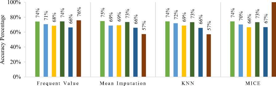
Figure 1 shows the accuracy of the classifiers on actual data. MICE imputation with the Deep Learning classifier gave 100% accuracy. While deep learning on KNN and mean imputation had only 57% accuracy. Frequent value imputation showed a slightly better accuracy at a range of 76%.

• ■    Random Forest

• ■    Gradient Boosted Tree

• ■    Decision Tree

• ■    Naive Bayes

• ■    Logistic Regression

• ■    Deep Learning

Imputation Techniques

Fig.1. Accuracy of classifiers on Actual Dataset

Figure 2 shows the accuracy of the classifiers on over-sampled data. Similar to Figure 2, the Accuracy of Mean imputation with Deep Learning classifier gave 100% accuracy, which was the peak accuracy. In KNN and MICE, accuracy was consecutively 83% and 81%. But Deep Learning produced only a 60% accuracy level on Frequent Value. Logistic Regression in every imputation showed only 66% to 70% accuracy.

• ■    Random Forest            ■ Decision Tree             ■ Logistic Regression

• ■    Gradient Boosted Tree      ■ Naive Bayes              ■ Deep Learning

  

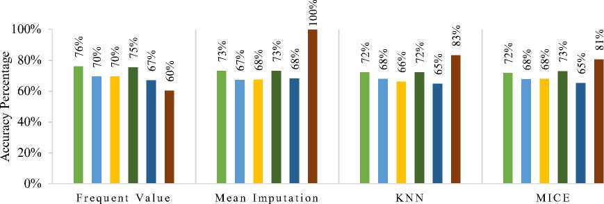
  Fig.2. Accuracy of classifiers on over-sampled dataset

  
  

• 6.2.    Classifier Performance based on Confusion Matrix

  In the actual data section (Table 3), Deep Learning in KNN has the least False Negative value, which is five. Also, Deep learning in Frequent Values has the Falsest Negative value, which is 1463. But Deep Learning has the least False Negatives if we compare it with all other classifiers. In comparison, Logistic Regression produced the greatest number of False Negative values overall. Logistic Regression was the worst performed classifier. In the over-sampled data section (Table 3), Deep Learning in KNN has the least False Negative value, which is seven. Naïve Bayes after Mean imputation has the most False-Negative value, which is 1250. Like the actual data, here, Deep Learning has the least False Negatives if we compare it with all other classifiers. In contrast, Logistic Regression produced the most False-Negative values overall. Logistic Regression was the worst performed classifier.

Imputation Techniques

Table 3. Confusion Matrix Values on Actual and Over Sampled Dataset

Imputation Technique	Classifier	Actual Dataset				Over Sampled
		True Positive	False Positive	True Negative	False Negative	True Positive	False Positive	True Negative	False Negative
Frequent Value	Random Forest	2696	928	2696	928	2704	940	2704	920
	Decision Tree	2470	1029	2470	1029	2465	1026	2465	1026
	Logistic Regression	2488	1136	2488	1136	2469	1155	2469	1155
	Gradient Boosted	2709	915	2709	915	2686	938	2686	938
	Naive Bayes	2396	1228	2396	1228	2402	1222	2402	1222
	Deep Learning	5747	1909	3565	1463	6709	4839	635	501
Mean Imputation	Random Forest	2838	968	2838	968	2837	969	2837	969
	Decision Tree	2547	1080	2547	1080	2577	1102	2577	1102
	Logistic Regression	2630	1176	2630	1176	2629	1177	2629	1177
	Gradient Boosted	2812	994	2812	994	2858	948	2858	948
	Naive Bayes	2516	1290	2516	1290	2556	1250	2556	1250
	Deep Learning	7178	5395	79	32	7201	5451	29	9
KNN	Random Forest	865	340	865	340	875	330	875	330
	Decision Tree	761	361	761	361	743	376	743	376
	Logistic Regression	1247	656	1247	656	1283	620	1283	620
	Gradient Boosted	882	323	882	323	890	315	890	315
	Naive Bayes	806	399	806	399	810	395	810	395
	Deep Learning	7205	5447	27	5	7203	5454	20	7
MICE	Random Forest	1364	539	1364	539	1383	520	1383	520
	Decision Tree	1178	641	1178	641	1215	573	1215	573
	Logistic Regression	1286	617	1286	617	1258	645	1258	645
	Gradient Boosted	1410	493	1410	493	1415	488	1415	488
	Naive Bayes	1287	616	1287	616	1268	635	1268	635
	Deep Learning	7199	5427	47	11	7197	5449	25	13

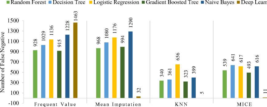
Figure 3 shows a visual representation of the difference between Confusion Matrix values of all classifications on actual data. In the previous accuracy percentage graph for every imputation technique, the Deep Learning classifier performs better than the other classifiers. Although it has around 1500 false negative values in Frequent Value imputation, judging by different Imputation technique’s False-Negative results with less than 30 in values for False-Negative, we can assume that frequent value imputation was not so effective.

Imputation techniques

Fig.3. False Negative Comparison between the Classifiers for the Actual Dataset

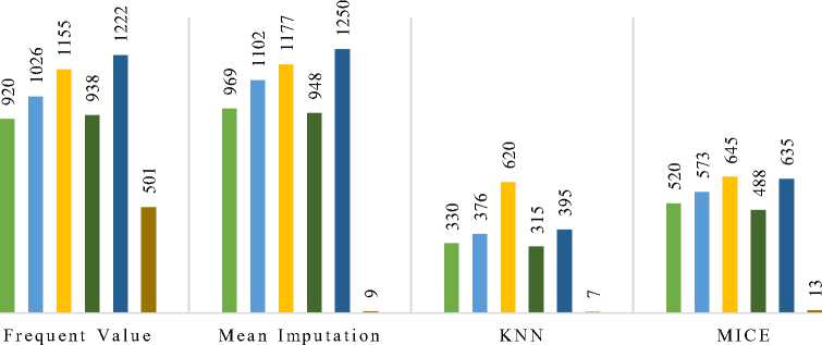
Figure 4 shows a visual representation of the difference between confusion matrix values of all classifications on over-sampled data. There are similarities between the last graph and this graph. Deep learning does better with the least false negative values in every aspect.

Random Forest ■ Decision Tree ■ Logistic Regression ■ Gradient Boosted Tree ■ Naive Bayes ■ Deep Learning

^ 1200

u 1000 z

^  600

z 200

Imputation Techniques

Fig.4. False Negative Comparison between the Classifiers for Over-Sampled Dataset

• 6.3.    Classifier Performance based on Coupon Type

7.    Conclusions

In the dataset, there are several types of coupons. Tables 4 & 5 took the column named “Coupon” and divided it into five sections along with the whole dataset. Bar. Coffee House, Restaurant <20, Restaurant (20-50), and Take-away; are the sections. After that, the complete process of imputation techniques and classification is done in each of the sections for every imputation and classification.

Table 5 shows a similar calculation as Table 4 but with oversampling of each of the different sections of the dataset. It is also seen here that the column “Restaurant (20-50)” has the least accuracy, with an average of 63.25%. Deep learning classifier did well in every column but gave a very mediocre result in column “Restaurant (20-50).”

Table 4. Accuracy of Classifiers Based on Coupon Type (Actual Data)

Imputation Technique	Classifier	Bar	Coffee House	Restaurant < 20	Restaurant (20-50)	Take Away
Frequent Value	Random Forest	74	75.4	75.9	62.7	73.4
	Decision Tree	72.6	72.8	67.1	59	72.7
	Logistic Regression	69.3	72.1	72.2	59.9	70.3
	Gradient Boosted Tree	73.3	75.2	75.4	66.9	71.9
	Naive Bayes	65.7	69.1	73	61	72.1
	Deep Learning	80.86	79.68	80.11	73.19	78.85
Mean Imputation	Random Forest	71.9	74.6	78	65.4	73.5
	Decision Tree	71.5	74.5	69.98	61.9	69
	Logistic Regression	69	71.4	76.2	66.7	71.3
	Gradient Boosted Tree	76.2	74.5	79.2	67.9	74
	Naive Bayes	68	70.2	76.4	66.5	67.5
	Deep Learning	69.86	64.69	73.40	66.62	71.96
KNN	Random Forest	73.4	70.3	75.1	62	75.4
	Decision Tree	66.7	69.3	67.8	52.7	70.9
	Logistic Regression	61.4	62	76.8	63.8	73
	Gradient Boosted Tree	76	72.4	75.5	61.3	75.9
	Naive Bayes	68.2	68.7	73.2	60.6	67.5
	Deep Learning	70.20	69.37	76.78	66.15	74.26
MICE	Random Forest	69.6	70.7	76.3	60.7	73
	Decision Tree	72.5	67.9	68.1	58	63.7
	Logistic Regression	62.7	56.5	72.2	66.1	68.8
	Gradient Boosted Tree	73.6	74	75.6	66.5	68.8
	Naive Bayes	70	72.3	75.8	64.7	69.6
	Deep Learning	67.77	65.37	76.99	57.76	73.72

Table 5. Accuracy of Classifiers based on Coupon Type (Over Sampled Data)

Imputation Technique	Classifier	Bar	Coffee House	Restaurant < 20	Restaurant (20-50)	Take Away
Frequent Value	Random Forest	78.2	78.5	76.7	67	77.6
	Decision Tree	76.5	75.6	66.1	64.3	72.4
	Logistic Regression	75.1	72.3	75.8	64.5	75.1
	Gradient Boosted Tree	79.2	78	78.8	67	75.8
	Naive Bayes	70.3	70.4	76.6	65.2	71.9
	Deep Learning	71.74	61.63	66.33	67.29	74.09
Mean Imputation	Random Forest	75.7	74.6	75.7	66.1	74.8
	Decision Tree	71.1	71.4	70.4	60.8	70.6
	Logistic Regression	73.8	70	77.8	65.2	68.9
	Gradient Boosted Tree	77.9	75.3	79.4	69	73.8
	Naive Bayes	71.8	66.3	77.5	63.8	65.7
	Deep Learning	69.46	63.71	70.78	63.81	57.06
KNN	Random Foresta	76	75.4	78.5	68	75.3
	Decision Tree	73.8	73.2	67.4	62	71.2
	Logistic Regression	70.8	72.4	75.8	63	70
	Gradient Boosted Tree	77.6	75.5	78.7	69.4	74.6
	Naive Bayes	70.3	66.7	76.4	60.9	66.5
	Deep Learning	71.15	67.97	74.48	67.29	57.01
MICE	Random Forest	74.6	76.4	76.7	61.2	74.1
	Decision Tree	73.5	69.9	67.5	64.1	69.5
	Logistic Regression	62.9	62.7	75.4	62.1	66.4
	Gradient Boosted Tree	77.9	74.4	77	64.3	73.5
	Naive Bayes	70.6	69.6	72.4	61.2	66
	Deep Learning	71.54	62.44	71.14	63.74	56.98

The significance of this study on the In-Vehicle Coupon Recommendation dataset is that it will help both the clients and the shops by predicting coupon recommendations correctly. The shop or store owners would be able to target their customers to give away coupons or offers. If the users take the vouchers, the company would be benefited from them. This is why proper prediction of the missing data is essential in this research. The accuracy of the prediction models helps to find out if the coupons are helpful or not. Finding missing data faultlessly was challenging because this dataset had many missing values. This dataset was also imbalanced by 57% positive and 43% negative instances. Four different imputation techniques were applied to this dataset to replace missing values. Those imputation techniques are Mice, Mean, KNN, and Frequent Value Imputation. To find out the accuracy of the imputation methods, classifiers were used. The classifiers that we have used are - Gradient Boosted Tree, Naive Bayes, Deep Learning (Keras), Logistic Regression, Random Forest, and Decision Tree. As the dataset was imbalanced, we applied SMOTE to oversample the dataset and run the whole process afresh on the oversampled dataset. Here, the accuracy of KNN was the highest of all. The survey shows that Deep Learning gave the least false negative (5) and the highest accuracy among all classifiers. The dataset showed accuracy up to 100% with the Mean imputation technique and Deep Learning classifier. These values show that balancing the dataset and implementing imputation techniques gives more accurate results. The Deep Learning classifier helped to achieve maximum accuracy. For comparing our results with an existing one, we have chosen the paper “IDA 2016 Industrial Challenge: Using Machine Learning for Predicting Failures". The winner scored 9920 points with 542 false positives and 9 false negatives in the IDA 2016 competition [16]. Using mean imputation along with Deep Learning classifier, our false-negative score is better than the best competitor in that competition. In the near future, focusing on imbalanced datasets, using more updated imputation techniques, and implementing updated Deep Learning classifiers might help get more accurate results.