A Concave Hull Based Algorithm for Object Shape Reconstruction

Author: Zahrah Yahya, Rahmita W Rahmat, Fatimah Khalid, Amir Rizaan, Ahmad Rizal
Journal: International Journal of Information Technology and Computer Science(IJITCS) @ijitcs
Article in issue: 3 Vol. 9, 2017.
Free access
Hull algorithms are the most efficient and closest methods to be redesigned for connecting vertices for geometric shape reconstruction. The vertices are the input points representing the original object shape. Our objective is to reconstruct the shape and edges but with no information on any pattern, it is challenging to reconstruct the lines to resemble the original shape. By comparing our results to recent concave hull based algorithms, two performance measures were conducted to evaluate the accuracy and time complexity of the proposed method. Besides achieving the most acceptable accuracy which is 100%, the time complexity of the proposed algorithm is evaluated to be O(wn). All results have shown a competitive and more effective algorithm compared to the most efficient similar ones. The algorithm is shown to be able to solve the problems of vertices connection in an efficient way by devising a new approach.
Convex hull, concave hull, vertices, shape reconstruction
Short address: https://sciup.org/15012623
IDR: 15012623
Text of the scientific article A Concave Hull Based Algorithm for Object Shape Reconstruction
Published Online March 2017 in MECS DOI: 10.5815/ijitcs.2017.03.01
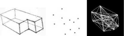
Many approaches are given to solve the problem of polygon computing to approximate geometric shapes based on a given point set in ℝ2 . Various methods are designed specifically based on the nature of the output [1]. The objective of this research, is to connect the points or vertices from the identified object faces that contain disordered vertices of (x, y). One of the challenging tasks is to know which vertices to connect together as we have no connectivity information. Typically, a line is drawn from each vertex to every other remaining vertex to form a polygon such as the OpenGL_Line ready function. However, this does not allow the recognition of the real object as can be seen in Figure 1. The main objective of the proposed method in this paper is to imitate the source drawing and reconstruct the shape. Given a set of points
(vertices) from two faces representing the dominant shape of the object, the goal is to connect them “connect-the-dots” by finding the correct path to produce a ‘meaningful’ object. The most relevant studies that could address this issue are the ones done on hull computation. Numerous algorithms were developed and improved over the years to address the problem of hull computation and detection [2]–[5]. The algorithm starts with the convex hull computation and several works developed from this process are still considered as state of the art. The strategies to solve the problem in this paper are taken as a basis on how to handle convex and non-convex objects.
(a) (b) (c)
Fig.1. A connection on (a) a sample object of our dataset, (b) vertices of the object and (c), Line drawing between points in OpenGL.
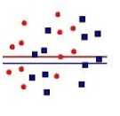
The computations of convex and concave hulls on the set of points in two-dimensional planes are still a challenge in many different areas. They have been widely used in many fields such as computer graphics, image processing, GIS, wireless tracking, pattern recognition and artificial intelligence. It is important to understand that numerous algorithms are designed based on very different needs. The construction of hull from a given set of points is used to detect convexity or concavity as can be seen in Figure 2. The convex hull of a point-set is the smallest convex space that contains all the points belonging to that set. For a finite 2D point-set, the convex hull can be defined as the smallest convex polygon containing all the points. Meanwhile, concave hull is described when the hull around one set of group of objects is not required to have a convex shape. The shape defined allows any angle between the points. Convex hulls have several useful properties that can be suitable for a variation of recognition and representation tasks. A convex hull can also be defined when the shape that contains all the points does not have any angle that exceeds 180 degrees between two adjacent points.
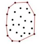
(a) Convex hull
(b) Concave hull
-
Fig.2. Classification of convex and concave hull. Adapted from [6]
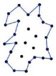
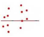
Graham’s scan algorithm [4] for computing the convex hull is used as a basic idea for connecting set of points in a plane. The result of convex hull construction using Graham’s Scan shows that the enumeration is to extract the extrapolation or the image boundary. The algorithm does not enumerate points with same x or y value and neglects the inner points. Figure 3 shows several results for using Graham’s Scan Algorithm. As seen in the figure, the convex hull technique does not reflect the original shape which mostly has a dataset of concave objects. Thus, concave hull is a better choice and is more advanced to capture the concaveness of the shape of the object [7].
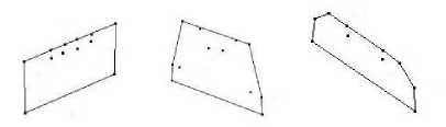
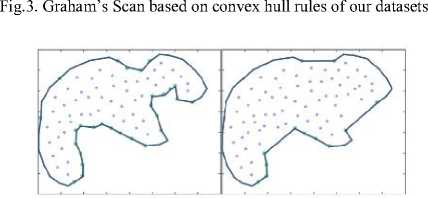
Fig.4. The smoothness of concave hull determined by threshold [7]
Concave hull computation is an active field in computation geometry with different approaches to compute the boundaries from point sets of the arbitrary shape. There are many known algorithms for computing convex hull but very few for computing concave hulls. The techniques used to compute concave hulls are based on nearest neighbor, kernel functions, using a convex hull or Delaunay triangulation. A prominent algorithm for concave hull computation is to construct non-convex or simple polygons that characterize the shape from a set of points in the plane. It is based on the Delaunay triangulation of the points. The method first creates a convex Delaunay triangulation with the entire vertex connecting each other. Then, the algorithm removes the edges that are smaller than a certain threshold value, but still does not give any expected results. However, it is not applicable in our work because the algorithm still connects the most outer points. The smoothness of the shape is based on the ‘digging method’ and threshold value in order to produce the appropriate depth as shown in Figure 4. In conclusion, we abandoned the convex hull approach because it cannot preserve the original object shape.
The challenge in this work is of how to re-implement hull based algorithms to utilize the concavity to reconstruct an object shape. While any convex and concave hull approach ignores some points, our work inspects all points for a given object to be connected. By comparing and analyzing the time complexity of the previous algorithms we have realized the issue of high time complexity. In this study, a technique for object shape reconstruction is proposed by utilizing a ‘splitting and recombination’ approach to correctly connect the vertices which also affects the detection of the object shape. We have emphasized on a design to decrease the time complexity in comparison with the best options. Point and vertex is used interchangeably throughout this paper.
This paper is organized as follows: section 2 presents the related works. Section 3 describes the concave Hull based algorithm developed for object shape reconstruction. Section 4 introduces the implementation undertaken. Section 5 presents some examples of the obtained results, and discusses performance evaluation of the implemented algorithm. Section 6 concludes with some remarks and future work.
-
II. Related Works
Computing a set of points in a plane to represent a shape has arisen in the computer vision and computer graphics domain. It has been used to solve several problems in pattern recognition, control theory, machine learning, computational graphics, and structural health monitoring and also signal classification. A shape recognized from a set of points can easily be perceived by a human brain, but the recognition is difficult for a computer. Before related works are presented, it is important to define the ideas about terminologies and the difference of opinion. There are several hulls, however we reviewed the concave hull category due to their wide and various range of utilization.
Duckham et al. [12] proposed a technique called x- algorithm to generate a characteristic hull-based method. They applied this method for boundaries shaping the countries and also alphabet letters using datasets of known distribution. The x-shape algorithm is based on Delaunay triangle which receives dot patterns as input and produces a polygon as an output. A length parameter l is introduced between the shortest and longest boundary edges. No digging can occur when the l is longer than the longest boundary edge. The concavity degrees rise when the edge is shorter than the shortest boundary edge. This method is to delineate the polygonal regions as an alternative to a minimum convex polygon (MCP) and is considered as one of the time-efficient concave hull algorithms with a time complexity of O(nlogn) [13].
Table 1. A time complexity comparison of concave hull algorithms
|
Algorithms |
Time complexity |
|
Galton & Duckham [1] |
0 ( n3 ) |
|
Moreira & Santos [11] |
0 ( n3 ) |
|
Duckham et al. [12] |
0 ( n log n ) |
|
Park & Oh [7] |
0 ( n log n + n ) |
|
Methirumangalath et al. [14] |
0 ( n log n ) |
-
III. The Proposed Methods
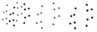
The aim of the algorithm is to create edges or connect unorganized vertices in each face (f2_ ) and (f2 ) and between the two faces in order to define the original shape. Figure 5 shows a set of vertices of an object comprising of two faces that provides no connection information. Each face is a representative of a side of a symmetric object.
(a) (b) (c)
Fig.5. Two-dimensional vertices represents an object: (a) object vertices, (b) vertices of face 1 (f) and (c) vertices of face 2 (f)
The proposed approach is based on the points or vertices which are elements of ℝ2 in the plane. The first step is to determine the Seed Point SP as the connection determinant for the initial and subsequent vertices construction. The second step is region splitting which is to divide the faces into two parts based on the centroid of the face vertices. In the third step, the vertices in each region are connected and complete face connection is completed in the fourth step where the edges are added between faces. The procedure used in this algorithm is illustrated in the flow shown in Figure 6.
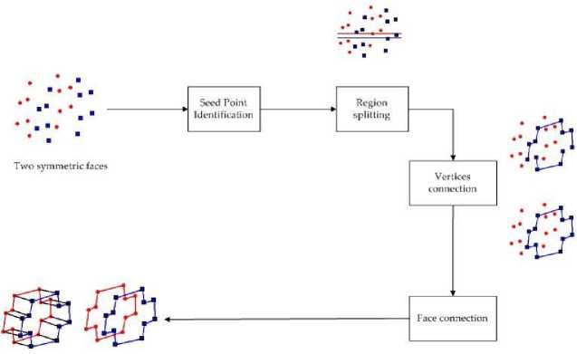
Fig.6. The procedure of the proposed method
-
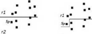
A. Seed Point Identification
This is the first stage where certain elements are determined for accurate shape identification. Based on our method, each face must be divided into two regions which are referred as the upper region (r^ ) and the lower region (r2) based on the centroid of the face vertices. The Seed Point (SP) is a starting point for connecting vertices and needs to be declared beforehand. If a wrong seed point is selected, it may result in misconnecting and thus produce the wrong shape. To determine the SP , a minimum x value is initialized and is resided in the first index of the upper region (r ), meaning that the regions would change to include the seed point at the upper region (r ) automatically. Later, the remaining vertices are computed for the region division. Figure 7 shows the seed point being dedicated to the upper region and the region classification represented in equation (1).
f ( SP )= х _ min ( Vi ) ⊩ 71 (1)
V =∑ "=1^/^ ,
wℎ ere W[ ∈ ℝ, Wi ≥0 for eac ℎ i
[ n ], ctnd ∑
∈
n wt=1 i=l
For every face, two regions are partitioned based on the centroid of y-axis or x-axis. In equation (3) we show that the remaining vertices which are less than Y (also same for X) are assigned to r and the rest are kept in r . The centroid of vertices in respect to Y are accumulated in the second equation of (3). The y-values of the vertices, yi for 0 ≤ i < n, are used to split the region into horizontal strips while x-values in vertical strips. Figure 8 illustrates the visualization of the object face with the division of two regions.
f( Г ) Vi +1 ∈ V1 , if (^l+l (У)≤ ̅) (3)
(Vi+1 ∈ 12 , else if (^l+l (У)> ̅) (3)
̅∑У/ wℎ ere : =
r2
(a) (b)
Fig.7. (a) The original location of seed point in (r) (b) Seed point (sp) being dedicated to the upper region (r)
Tl
(a) (b) (c)
Fig.8. (a) An imaginary lines shows the centroid of (b) f and (c) f that splitting the regions
-
B. Region Splitting
There are two sets: face f! and f2 containing all the vertices v ,v2,…,vn corresponding to the object which is also expressed in equation (2). The algorithm is to find the upper region (r ) and lower region (r2 ) based on the remaining vertices after seed point has been identified. Later these two regions are merged together in order to have complete connection in the object face.
-
C. Vertices Connection
The idea of traversal strategy between vertices in this phase is based on an incremental construction approach which is a method of computing the convex hull of a finite set of vertices. While convex hull method chooses the anchor point from the lowest y coordinate, the algorithm sets the least x coordinate as the starting point. To reduce the complexity of the disorganization, the connection is broken into two regions which are upper region (r^ ) and lower region (r2 ) as described in the previous section. The algorithm is operated by a “walking” procedure. It walks clockwise for upper regions while counterclockwise for lower regions.
For a formulated description of the procedure, let SP be the point in r with the minimum x - coordinate or the leftmost vertex and let (v2,v2,…,vи) be the remaining vertices in r^ . Starting from SP, the connection is made based on x+ direction until the rightmost vertex. This is explained in equation (4) where we start from our seed point SP and by incrementally differentiating the x values. The same procedure is performed on the lower region but with the exception of the direction. In case the next two vertices to be connected have the same x value, the smallest angle of the vertex is chosen based on equation (5), where Atan2 is to find angle in radians between two points ( δy, δx) . After each of these two regions is complete, they are concatenated into a complete face by connecting the corresponding first and last vertex in both regions.
( Vc)=SP +∑(Xi - Xi-1)∶ SP = ,X ∈(a,b], n∈ ℤ+ i=2
8y = 2- У 1
8x = 2- X 1
angle =| Atan 2( 8y , 8x ) ∗ (^)| (5)
Figure 9 shows the process of creating a combination of faces as a result of the algorithm. In Figure 9 (a) two regions of f are shown which will be unified to a single face in figure (b). The same is shown for the f2 in figure (c) and figure (d). Figure (e) shows the combination of the faces together as the result of our algorithm for this
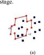
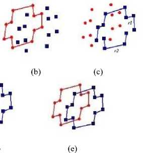
Fig.9. (a) Two regions of face one (b) the unified single face one (c) two regions of the second face (d) the unified single face two (e) the connection of each face
-
D. Face Connection
In continuance of the previous step, every vertex of a face is connected to form the original shape. The results for now would be in a 2D form. To achieve the complete object, these faces are connected. New edges are inserted to each corresponding vertex of each region and face as shown in Figure 10.
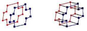
Fig.10. The two faces is concatenated for a complete geometric object
-
E. Overall Algorithm
Input: Face Vertices //Two faces of the object contain same number of vertices
Result: Polygon/object connection //Set of edges form object shape
/*1. List Initialization*/
The whole list is sorted (radix sort) as two arrays: X -array and У -array
/*2. Seed Point Identification*/
The minimum x value from the X -array is initialized as the
Seed Point ( SP )
The ( SP ) is resided as the first index in the X -array
/*3. Region Splitting*/
Get the centroid of У - axis of the vertices from У -array
FOR all of the vertices I
IFF(I)≤centroid vertex ∈ ri
ELSE vertex ∈ r2 end FOR
/*4. Vertices Connection*/
The walking procedure is based on the x+ - direction and the smallest angle between two vertices ( X ( i ), X ( i +1))
//clockwise for f i and counter clockwise for F 2
We start from SP and go one by one through the X -array.
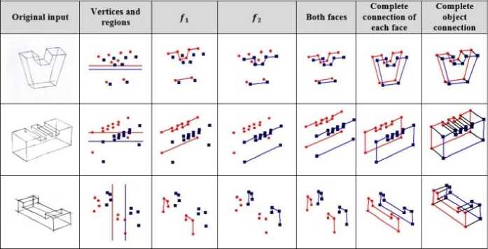
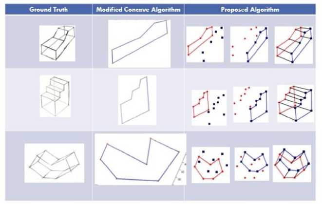
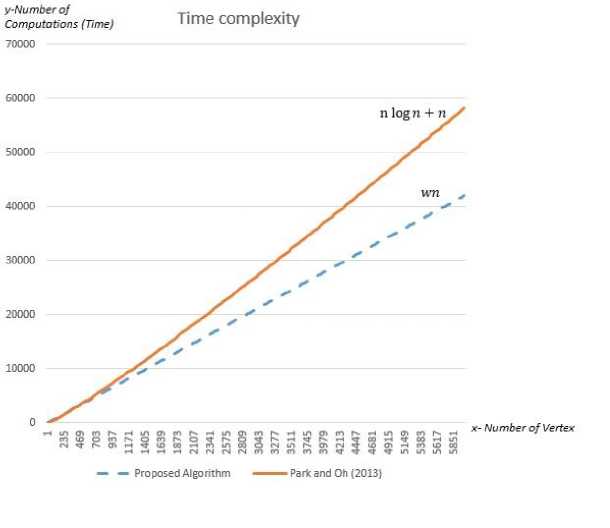
FOR all of the t in the г i and ^*2 of X-array tfX(i) Insert new edge (i,I+1) if X (i)=X(i+1) if angle (X(i))<angle (X(i+1)) Insert new edge (i,i+1) end FOR Connect the first index of F J to the first index of ^* 2 and Connect the last index of F J to the last index of ^" 2 /*5. Face Connection*/ The connection is based on the clockwise movement FOR all of the vertices i Insert new edges (Fl → ^" 1 (i), F2 → ri (i)) Insert new edges (Fl → ^*2 (i), F2 → r2 (i)) end FOR Fig.11. The proposed pseudo code for object shape reconstruction IV. Implementation A Graphical User Interface (GUI) is designed to run the entire algorithm and to test the experiments for producing the results. The data structure and coded blocks were built based on each process indicated in the proposed methodology section. The implementation is to ensure that the overall algorithm is efficient enough to connect the vertices within the faces and to connect both faces accurately. Visual Basic 6.0 has been chosen as the development environment at this stage. Figure 12 shows the system GUI for object shape reconstruction process. The elements of each process have been segregated to show the progress in each stage for algorithm validation. In the top left corner it shows the visualized raw data as input and through the stages it reaches to the bottom right corner, visualizing the overall model as a result. Fig.12. The system interface for object shape reconstruction algorithm for a sample object from our dataset V. Experiments, Results and Discussion The object shape reconstruction algorithm can successfully obtain its objective in constructing the final shape from two set of faces with disorganized vertices. As explained in the introduction of this chapter, there are several experiments which have attempted to solve the connection problem. A challenge for all of these studies is to find the connection as there is no clue about how the points should be connected. Generally, the connections between vertices are made through incremental construction based on the x axis and angle evaluation for each prior vertex to the next vertex. These connections between the set of points should preserve the original shape of the object. We name the technique as the splitting and recombination technique due to the reason that we first split the vertices and then recombine to create the shape. It is used to gratify the process of the connection. A sample of the experiment results are presented in Table 2. Table 2. Sample output of the vertices connection experiments To evaluate and validate the proposed object shape reconstruction algorithm, experiments are conducted on a computer with specifications of Windows 7 Professional, 8G-RAM and 3.2 GHz CPU. We have also gone through a series of performance evaluations to make sure that the proposed algorithm is precise and correct. We evaluated the accuracy of the output and computational/time complexity by modeling the computation/time usage of the proposed algorithm. This would give us estimates to know how fast the algorithm could deliver the output if the numbers of vertices which are the inputs are considerable. A. Performance Evaluation (Accuracy) One of the metrics evaluated is the accuracy of the proposed algorithm. The performance of the proposed algorithm is evaluated against the well-known concave hull algorithm based on the precision metric. Precision can be defined as the exactness of measurement. Equation (6) is used to compute the precision: Precision = (6) TP+FP v 7 Let TP (True Positive) represent the correct shape detected. FP (False Positive) is when we are unable to detect the true or correct shape (falsely detect). Our algorithm does not include a method to detect false or incorrect shapes. The algorithm either detects a correct shape (TP) or does not detect (FP) by its inefficiency. Based on this description there is no recall to be estimated. We defined the accuracy which is the closeness of a measurement to the true value and could conclude the precision we reach as accuracy. The more precise the proposed algorithm detects the shapes, the more accurate it is. Fig.13. A sample visual comparison of the results between ground truth images, modified concave algorithm and the proposed algorithm B. Performance Evaluation (Time Complexity) The time complexity models the time taken by an algorithm as the input size rises considerably. It is usually expressed using the big O notation to classify algorithms by how they performed on input data size they are working on [15]. It is measured by estimating the number of elementary operations performed by an algorithm; either in loops or other functions. Based on the evaluated model, the algorithm could be compared with other algorithms to determine the most efficient in terms of the time or computations needed to finish the entire process. 2-dimensional dataset. It utilizes a convex hull algorithm to generate a list. Convex hull has a O(nlogn) complexity. For the next three steps the algorithm digs through the concave list. The authors have mentioned that the overall complexity of their algorithm is O(nlogn). Referring to our algorithm in Figure (11), we show 5 distinct stages. We computed the complexity of each stage and conclude as follows: T1: List initialization: Radix Sort has been used to sort the entire list due to its efficiency. Normally Radix Sort complexity is computed by: O(wn) where w is our word size. (For example 123 has a word size of 3 while 23 has a word size of 2 because of the number of digits composing the number). In our case, the vertices are not scattered in long distance and so our word size w might not even exceed 3. T2: Seed point identification: Simple initialization, O(1) T3: Region splitting: Goes through the whole list and assigns based on centroid O(n) T4: Vertices connection (Walking): Walks through all the edges using the x-array, O(2n) T5: Face connection: Goes once through all the vertices and inserts edges, O(n) Therefore, the total estimated time complexity is O(wn) where w is estimated to be between 7 and log(n). In the worst case scenario where are vertices are scattered in very far apart distances the time complexity would reach O(nlogn) but it would still be smaller. This is far from possible based on the nature of our work. Based on mathematical evidence, O(wn) has less complexity in comparison with O(nlogn + n) by Park and Oh [7]. A graph shown in Figure 14 shows a visual comparison of the complexities of the two algorithms when many vertices are given as inputs. The y axis represents the number of computations which each computation is a unit of time. The x axis represents the number of vertices given as input to both algorithms. Fig.14. A time complexity comparison of the proposed algorithm with [7] VI. Conclusion This proposed algorithm producing the correct shape on finite vertices of a face object has several advantages. The main advantage is that the final procedure could accurately and efficiently complete the automatic reconstruction of object from sketch. It is also an automated algorithm with no user intervention required through the whole process of object shape reconstruction. In addition, to get the final output only a second of time is needed for our examples. This is due to the O(wn) computation/time complexity of the proposed algorithm. The computation/time complexity model shows that the proposed algorithm is more efficient in this aspect compared to any available concave hull algorithm. The lines are also accurately identical to the original object because the edges are drawn based on the vertices. One limitation is that the algorithm is highly dependent on accurate vertex detection. If a vertex is missed then the resulting shape would not produce the actual model.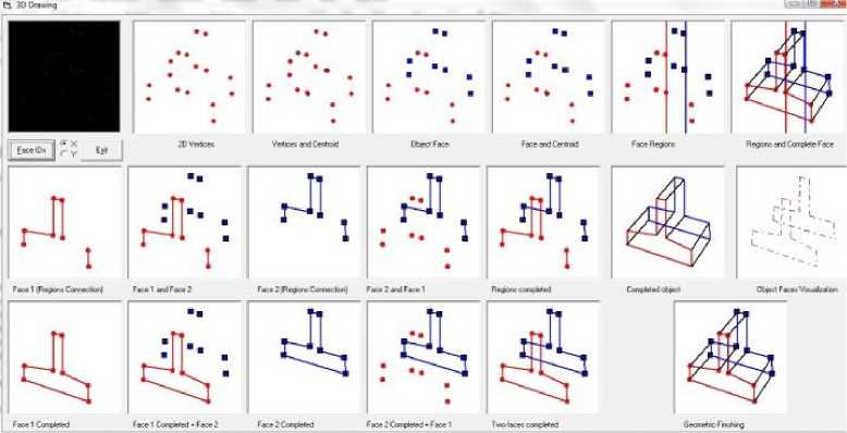
References A Concave Hull Based Algorithm for Object Shape Reconstruction
- A. Galton and M. Duckham, “What is the region occupied by a set of points?,” in Geographic Information Science, Springer, 2006, pp. 81–98.
- T. M. Chan, “Optimal output-sensitive convex hull algorithms in two and three dimensions,” Discrete Comput. Geom., vol. 16, no. 4, pp. 361–368, 1996.
- K. L. Clarkson and P. W. Shor, “Applications of random sampling in computational geometry, II,” Discrete Comput. Geom., vol. 4, no. 1, pp. 387–421, 1989.
- R. L. Graham, “An efficient algorith for determining the convex hull of a finite planar set,” Inf. Process. Lett., vol. 1, no. 4, pp. 132–133, 1972.
- R. A. Jarvis, “On the identification of the convex hull of a finite set of points in the plane,” Inf. Process. Lett., vol. 2, no. 1, pp. 18–21, 1973.
- E. Rosén, E. Jansson, and M. Brundin, “Implementation of a fast and efficient concave hull algorithm,” 2014.
- J.-S. Park and S.-J. Oh, “A new concave hull algorithm and concaveness measure for n-dimensional datasets,” J. Inf. Sci. Eng., vol. 29, no. 2, pp. 379–392, 2013.
- T. Ebert, J. Belz, and O. Nelles, “Interpolation and extrapolation: Comparison of definitions and survey of algorithms for convex and concave hulls,” in Computational Intelligence and Data Mining (CIDM), 2014 IEEE Symposium on, 2014, pp. 310–314.
- H. Edelsbrunner, D. G. Kirkpatrick, and R. Seidel, “On the shape of a set of points in the plane,” Inf. Theory IEEE Trans. On, vol. 29, no. 4, pp. 551–559, 1983.
- M. Melkemi and M. Djebali, “Computing the shape of a planar points set,” Pattern Recognit., vol. 33, no. 9, pp. 1423–1436, 2000.
- A. Moreira and M. Y. Santos, “Concave hull: A k-nearest neighbours approach for the computation of the region occupied by a set of points,” 2007.
- M. Duckham, L. Kulik, M. Worboys, and A. Galton, “Efficient generation of simple polygons for characterizing the shape of a set of points in the plane,” Pattern Recognit., vol. 41, no. 10, pp. 3224–3236, 2008.
- S. Meintjes, “Multi-objective optimisation of a commercial vehicle complex network,” University of Pretoria, 2013.
- S. Methirumangalath, A. D. Parakkat, and R. Muthuganapathy, “A unified approach towards reconstruction of a planar point set,” Comput. Graph., 2015.
- I. Chivers, J. Sleightolme, "An Introduction to Algorithms and the Big O Notation", Introduction to Programming with Fortran, Springer, 2015, pp.359-364
