A Density Control Algorithm For Wireless Sensor Network

Recent rapid advances in microelectronic and wireless communication have made it possible to integrate microsensor, low-power signal processing, computation and low-cost wireless communication into a sensor node. Wireless sensor networks consist of large number of sensor nodes which are scattered over a region of interest and has a feature of multi-hop communication[1].

If all nodes of a sensor network worked simultaneously, not only there would be a lot of redundant information, but also they would have great adverse impact on network throughput, bandwidth, latency, energy and network lifetime. Therefore, we can use density control technology to reduce the number of active sensor nodes under the precondition of ensuring network coverage and network connectivity. In this paper, we propose SNDC (Sensor Network Density Control), a density control algorithm for wireless sensor network to keep as few as possible sensors in active state to achieve the complete connected coverage of a specific monitored area. Inactive sensors can turn off sensing modules to save energy. Unlike other algorithms, this algorithm does not

This paper is supported by Preparatory Research Project

(9140A16020309HT01); Harbin Technology Innovation Project

(2009RFLXG009); The International scientific cooperative research program of China (2010DFA14400)

* Corresponding author.

rely on position information or ranging information of sensors. It just requires each active sensor to periodically send three beacons of different transmission ranges. Sensors can decide to stay active or inactive state according to received beacons. The proposed algorithm is fault-tolerant in the sense that one or more inactive sensors can switch to the active state to take over the surveillance responsibility when any active sensor runs out of energy or fails. Under the assumption of R_C ≥2 R_S , the algorithm can approximate the optimal connected coverage, where R_C and R C are the radio communication radius and the sensing radius of sensors, respectively.

The remainder of this paper is organized as follows. Related research efforts are discussed in section 2. The algorithm details of SNDC are given in section 3. Section 4 presents the simulations and results obtained. Section 5 concludes the paper.

• 2.    Related work

Density control algorithm can be classified into location-based algorithm and location-free algorithm by whether knowing its accurate location information.

Location-based algorithm, such as OGDC[2], tries to achieve connected coverage with a minimal number of sensors under the assumption that sensor locations and boundary information are known in advance. However, due to the cost and volume, node’s location information is often hard to know. Location-free algorithm is necessary for sensor networks accordingly.

Location-free algorithm can be classified into range-based algorithm and range-free algorithm by whether knowing its distance to other nodes. Some location-free and range-based algorithms are present in [3, 4, 5, 6]. They all use some ranging technology, such as RSSI[7], to get ranging information.

In the algorithm presented in [3], every node keeps a neighbor list and a 'co-worker' list. The neighbor list keeps the ID and an estimated distance of its neighboring sensor. The co-worker list keeps the ID of known active sensors. Initially, all sensors are in role-deciding state and a stochastic procedure is used to make some sensors become starting sensors, which would send out a co-worker request message attached with a co-worker list. According to the co-worker message received, the distances of senders and the receivers can be estimated by the RSSI scheme. Then a sensor can decide whether to reply to the message according to the relationship of the neighbor list, the co-worker list and the distance information. Sensors can then decide to keep active or inactive by the replying messages.

In the algorithm presented in [6], all sensors are inactive initially. A random backoff mechanism is used to select sensors which will become active sensors. Active sensors should broadcast working messages and use RSSI technique to measure the distance between two neighboring starting sensors, which in turn is used to determine the intersection statuses of active sensors.

However, ranging technique is error-prone since it is vulnerable to environmental interference and multi-path fading, etc. Consequently, range-free algorithm is more suitable for sensor networks. Some range-free algorithms are presented in [8, 9, 10]. PEAS in [8] uses a probing mechanism for a sleeping sensor to periodically wake up to broadcast a probe message to decide whether to change the state. If there is a reply from a working sensor, the probing sensor goes back to sleep, otherwise, it becomes a working sensor. Two probabilistic algorithms in [9, 10] relies on stochastic process for density control. Although location-free density control algorithms may not achieve complete coverage, they are very useful for sensor networks where sensors have no location information.

Some algorithm also assume the relation of sensor radio communication radius R C and sensor sensing radius R S . The paper [11] assumes R C = R S . It pursuits almost optimal complete coverage by strip-based deployment under the assumption of R C = R S . The paper [12] proves that the coverage of an area implies the connectivity of the sensors covering the area if R C ≥2 R S . It is a well-known result that the regular hexagon-based deployment (see Figure 1) can reach complete coverage with the optimal (least) number of sensors [13]. Therefore, under the consumption of R C ≥2 R S , this paper presents a density control algorithm which chooses active nodes to build an approximate regular hexagonal network structure and to achieve the complete network coverage. .

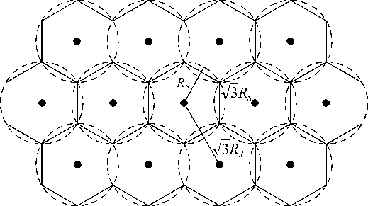
Fig. 1 The optimal deployment for the connected coverage of a monitored area

• 3.    Sensor Network Density Control Algorithm

  • 3.1.    Term Definitions

According to whether to monitor the network and transmit packets, sensor node's state can be classified into two kinds.

Definition 1 Active state

If a sensor node needs to open its transmitter to monitor the network and transmit the packets all the time, this sensor node's state is active state.

Definition 2 Inactive state

If a sensor node does not need to open its transmitter to monitor the network and transmit the packets all the time and can sleep periodically, this sensor node's state is inactive state.

Figure 2 shows the transferring graph of these two states.

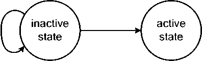
Fig. 2 Node state transferring graph

Definition 3 Sensing area

A node' sensing area is described as the rotundity area whose center is this node and radius is R_S .

Definition 4 Covered node

Covered node is defined as the node which located in the sensing area of an active node.

Definition 5 Uncovered node

Uncovered node is defined as the node whose location is not in the sensing area of any active nodes.

• 3.2.    Three beacons

  

• 3.3.    Sensor Network Density Control Alogrithm

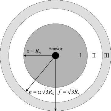
Fig. 3 Three beacons

In order to achieve the optimal hexagonal structure and complete network coverage, this algorithm uses three different beacons which have different transmission ranges: 3RR S for the f-beacon, 03R S for the n-beacon and R S for the s-beacon, where R S is the sensing radius and (1/^3) <  a <  1 (see Figure 3). In SNDC, the distance DIST between two neighboring active nodes must satisfies аТ3R_S <  DIST <  3RR_S , consequently, we can use f-beacon and n-beacon to achieve the approximate optimal hexagonal network structure (see Figure 4). S-beacon is used to have the complete network coverage.

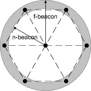
Fig. 4 Hexagonal structure formed by active nodes

This algorithm is composed of two phases. During the phase 1, we use n-beacon and f-beacon to build a hexagonal structure. During the phase 2, we use s-beacon to achieve the complete network coverage.

• 1)    The establishment of hexagonal structure

Initially, all sensor nodes are inactive and uncovered. A sensor node will monitor the network environment and then decided whether to participate in the establishment of hexagonal structure and change to an active node.

• (1)    Firstly, sensor nodes will receive beacons during the listening cycle T cycle , and decide whether to go to (2), (3), (4) based on the beacons they received.

• (2)    If a sensor node didn't receive any beacons during the T cycle , there is no active node near this node and it may become an active node. Because there might be some another nodes with the same situation near this node, backoff mechanism is needed to guarantee the unique active node in one sensing region.

Firstly, the node will choose a backoff time t randomly and backoff window is T backoff , t ∈ [0, T ] , and then begin to listening. If it didn't receive any beacons or only receive f-beacon by the end of t , node will become an active node and begin to periodically broadcast three types of beacons: n-beacon, f-beacon and s-beacon with interval T beacon till the death of energy exhaustion. Otherwise, node will go to phase 2.

• (3)    If the node only received f-beacon during the T cycle , it means that the node is located in the sectioni n of figure 3 and may become an active node which can build a hexagonal structure with other active nodes. Like (2), in order to avoid all these possible nodes become active, backoff mechanism is needed.

This node will choose a backoff time t randomly and backoff window is T backoff , t ∈ [0, T ] , and then begin to listening. If it didn't receive any beacons or only receive f-beacon by the end of t , node will become an active node and begin to periodically broadcast three types of beacons: n-beacon, f-beacon and s-beacon with T_beacon till the death of energy exhaustion. Otherwise, node will go to phase 2.

• (4)    If the node receives n-beacon during the T cycle , it means that the node is located in the section П of figure 3 and there is an active node near it. Consequently, this node will keep inactive and go to phase 2.

After this phase, an approximate hexagonal structure is built in the network.

• 2)    The repair and maintenance of Hexagonal structure

Because the approximate hexagonal structure built in phase 1 can not guarantee the complete network coverage, the repair and maintenance of hexagonal structure is necessary. In SNDC, all nodes which can not become active nodes in phase 1 will come into this phase 2. During this phase, the node will test whether it is covered by an active node. If not, whether it can become an active node and cover the network area nearby.

• (1)    Firstly, sensor nodes will receive s-beacons during the listening cycle Tcycle,.

• (2)    If the node received s-beacon during the Tcycle, it means that this node is covered by an active node. This node will remember the active node’s information and transmitting time, and then sleep. The node will wake up before the next s-beacon coming. This progress will repeat till its death of energy exhaustion or not receiving s-beacon. If this node didn’t receive any s-beacon, this node will go back to phase 1.

• (3)    If the node didn't receive any s-beacons during the Tcycle, it means that this node isn’t covered by any active node and may become an active node. In order to avoid all these possible nodes become active simultaneously, backoff mechanism is needed.

• 4.    Simulations and Results

• 4.1.    Simulation environment

  The following is the parameters used in the simulations. The communicating radius ( R C ) of each sensor is 200 meters and the sensing radius ( R S ) of each sensor is 100 meters. The backoff interval, beacon interval and listening interval of SNDC are 20 seconds. The working/sleeping ratio of Random Sleep algorithm is 50%, and the working cycle is 20 seconds. Transmission speed is 100kbps. We use IEEE 802.11 as MAC protocol. In the first simulation experiment, there are 500 nodes randomly deployed in a 500m×500m region (see figure 5). Each node of two algorithms can work for 200 seconds. In the second simulation experiment, we randomly deploy 1000 nodes in a 1000m×1000m region with α = 0.7, 0.8, 0.9. Each simulation runs for 10 minutes.

• 4.2.    Results and Discussion

  SNDC

  Random Sleep

  
  

Firstly, the node will choose a backoff time t randomly, t ∈ [0, T_backoff ] , and then begin to backoff. If it didn't receive any s-beacons by the end of t , node will become an active node and periodically broadcast three types of beacons: n-beacon, f-beacon and s-beacon with T beacon till the death of energy exhaustion. Otherwise, node will go back to (2).

After this phase, all network area will be covered by the active node as long as the network can be completely covered before density control. In order to guarantee every node can receive beacons during the backoff process, T backoff = T beacon = T cycle .

We have simulated the SNDC by OPNET modeler. Firstly, we compare the SNDC and the Random Sleep algorithm[14] in order to evaluate their effect on network lifetime. Secondly, so as to explore SNDC’s effect on network structure, we test some parameters of hexagonal structure related to α , such as the number of active nodes in hexagonal structure, their coverage area and coverage ratio.

Fig. 5 Simulation scenario

£   350

I 250

0ч—■—।—■—।—■—।—■—।—■—।—■—।—■—।—■—।—■—।—■—।—■—।—■—।

0   50 100 150 200 250 300 350 400 450 500 550 600

time (s)

Fig. 6 Simulation result of alive node number

Our first objective is to show that SNDC can increase the number of alive nodes and prolong the network lifetime. Figure 6 shows that SNDC can provide more alive nodes than Random Sleep algorithm and the number of alive nodes is more stable when network runs. This is mainly because that when an active node is chosen by SNDC, it will work till energy exhaustion and the network structure is stable during this period. Random Sleep algorithm choose a great deal of active nodes randomly which may change to sleep state after a working cycle. Consequently, Random Sleep algorithm has an unstable network structure and less number of alive nodes.

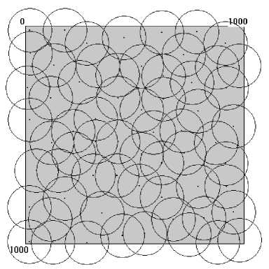
Fig. 7 Covered network of active nodes selected by SNDC

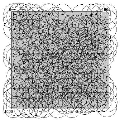
Fig. 8 Covered network of active nodes selected by Random Sleep

Table 1 Simulation results

α	Number of active nodes before phase 2	Coverage ratio before network repair	Number of active nodes after phase 2	Coverage ratio after network repair
0.7	49	95.0283%	67	100%
0.8	39	90.5367%	64	100%
0.9	32	82.5248%	65	100%

Our second objective is to show that SNDC can decrease the number of active nodes. Figure 7 and figure 8 shows two algorithms' active nodes and their coverage area at 50 seconds. At this time, SNDC chooses 63 active nodes which can cover 99.16% network area and Random Sleep chooses 259 active nodes which can cover 99.88% network area. This is mainly because when SNDC choosing an active node, distance between two nodes is taken into account, which can decrease the number of active nodes remarkably.

Table 1 shows the number of active nodes and coverage ratio before/after network repair in the second simulation experiment. Simulation results show that SNDC selects small active nodes to cover the complete network and it chooses more active nodes when α is small.

• 5.    Conclusion

In order to reduce the number of working sensor nodes and prolong the network lifetime, density control technique is necessary for wireless sensor networks. Under the consumption of RC≥2RS, this paper presents a sensor network density control algorithm SNDC which chooses small active nodes to build an approximate regular hexagonal network structure and achieve complete network coverage. In this algorithm, every active node needs to periodically send three beacons of different transmission ranges: n-beacon, f-beacon and s-beacon. N-beacon and f-beacon are used to build the hexagonal structure. S-beacon is used to achieve the complete network coverage. Inactive node can sleep to save energy and change to an active node when its former active node failed. Therefore, this algorithm is fault tolerant. Simulation results show that this algorithm can prolong the network lifetime and guarantee the small number of active nodes and the complete network coverage.