A Growing Evolutionary Algorithm and Its Application for Data Mining

Author: Ning Hou, Zhanmin Wang
Journal: International Journal of Intelligent Systems and Applications(IJISA) @ijisa
Article in issue: 4 vol.3, 2011.
Free access
An unsuitable representation will make the task of mining classification rules very hard for a traditional evolutionary algorithm (EA). But for a given dataset, it is difficult to decide which one is the best representation used in the mining progress. In this paper, we analyses the effects of different representations for a traditional EA and proposed a growing evolutionary algorithm which was robust for mining classification rules in different datasets. Experiments showed that the proposed algorithm is effective in dealing with problems of deception, linkage, epistasis and multimodality in the mining task.
Association rule, evolutionary algorithm, representation
Short address: https://sciup.org/15010191
IDR: 15010191
Text of the scientific article A Growing Evolutionary Algorithm and Its Application for Data Mining
Published Online June 2011 in MECS
Evolutionary algorithms (EAs) are robust adaptive systems that have been applied successfully to hard optimization problems [1,2,3]. There are two famous approaches commonly used by evolutionary algorithms as classifier systems, the Michigan approach and the Pittsburgh approach [4]. The Michigan approach maintains a population in which each individual is a rule and the Pittsburgh approach maintains a population in which each individual is a rule set and is encoded as a variable-length string.
Both of the two approaches run under the standard framework of EA and are based on the assumption that the fitness function value can be used to estimate the distance to the nearest global maximum. However, a lot of factors existed in the process of searching for associative rule largely affect the result of optimization, for example, linkage, epistasis, multimodality and deception [5,6]. How to eliminate these affections has become a key problem when the evolutionary algorithms were used in data mining. In this paper, we propose a growing evolutionary algorithm (GEA) for data mining which can be used to decrease the disturbances coming from deception, linkage, epistasis and multimodality.
-
II. realted work
A. GA Difficulty
The search for factors affecting the ability of the GA in optimization problems has become a major focus within the theoretical GA community. The two key problems preventing GA from finding the global optima efficiently are deception and linkage [7]. According to schema theorem and building block hypothesis, proposed by Holland, it is very hard for a high order schemata or building blocks to be recombined by low order ones in population-based searching [8]. This will result in an inefficiency implementation of traditional GA. Based on the work of Bethke [9], Goldberg proposed several approaches to deal with this kind of problems [10,11]. At the same time, a new crossover operator has also been proposed by Harik [12] to evolve the tight linkage. Das [13] claimed that deception is the only thing that is important in making a problem hard for a GA. However, Grefenstette [14] believed that deception is neither necessary nor sufficient for a problem to be hard for a GA. Now, it is clear that all of the facts, linkage, epistasis, multimodality, noise, deception and spurious correlations, can cause difficulty for a GA.
A model of fitness landscapes developed by Jones [15] suggests that there are strong connections between GA search and heuristic search. A general principle of heuristic functions is that they should correlate well with the distance to the goal of the search. If the fitness function of GA is viewed as a heuristic function, the value of fitness function is the estimate distance to the nearest goal of the search. FDC is a method of quantifying the relationship between fitness and distance.
Given a set F={f1, f2, …, fn} of n individual fitness values and a corresponding set D={d1, d2, …, dn} of the n distances to nearest global maximum, we compute the correlation coefficient r, as r=cFD/sFsD, where
n cFD=1∑fi-f)(di-d) n i=1
is the covariance of F and D, and s F , s D , f and d are the standard deviations and means of F and D respectively.
This work was supported by the National Natural Science Foundation of China (Grant nos. 60743009)
B. Association Rule and Associative Classification
Let τ={i1,i2,…,im} be a set of literals, called items. Let D be a set of transaction, where each transaction T is a set of items such that T ⊆ τ. Formally, an association rule R is an implication X => Y, where X and Y are sets of items or itemsets in a given dataset. The confidence of the rule Conf(R) is the percentage of transactions that contain Y amongst the transactions containing X. The support of the rule Supp(R) is the percentage of transactions containing X and Y with respect to the number of all transactions. Given a set of transactions D, the problem of mining association rules is to generate all association rules that have support and confidence greater than the user-specified minimum support ( called minSuppport ) and minimum confidence (called minConfidence) respectively [16].
Supp(R)>=minSupport (1)
Conf(R)>=minConfidence (2)
Liu [17] first proposed the AC approach, named classification based on associations algorithm (CBA), for building a classifier based on the set of discovered class association rules (CARs). The difference between rule discovery in AC and conventional frequent itemset mining is that the former task may carry out multiple frequent itemset mining processes for mining rules of different classes simultaneously.
Assuming that a dataset is a normal relational table which consists of N cases described by t distinct attributes, we can treat a case as a set of (attribute, integer-value) pairs and a class label. Each (attribute, integer-value) pairs can be called an item. Data mining in associative classification (AC) framework usually consists of two steps:
-
(1) Generating all the class association rules (CARs) which has the form of iset => c, where iset is a set of (attribute, integer-value) pairs and c is a class.
-
(2) Building a classifier based on the generated CARs. Generally, a subset of the association rules was selected to form a classifier and AC approaches are based on the confidence measure to select rules.
-
III. GA DIFFICULTY IN ASSOCIATION RULE MINING
A. The Different Representations of Rules in Rule Space
In this section, we describe a dataset D which consist of four condition attributes A={a1,a2,a3,a4}, B={b1,b2,b3,b4}, C={c1,c2,c3,c4}, D={d1,d2,d3,d4} and a class attribute E={e1,e2}. Each attribute contains four values and we represent them with five variables X, Y, Z, M and N as follows:
x=1 → a1, x=2 → a2, x=3 → a3, x=4 → a4 y=1 → b1, y=2 → b2, y=3 → b3, y=4 → b4 z=1 → c1, z=2 → c2, z=3 → c3, z=4 → c4 m=1 → d1, m=2 → d2, m=3 → d3, m=4 → d4, n=1 → e1, n=2 → e2
As can be seen in Fig.1-A, we describe a record of the dataset D with a circle. The yellow circles are records in class e1 and the green ones are records in class e2.
However, if we change the representation of the record, we can obtain another distribution of the records in record space, which can be seen in Fig.1-B.
x=1 → a1, x=2 → a4, x=3 → a3, x=4 → a2 y=1 → b1, y=2 → b3, y=3 → b4, y=4 → b2 z=1 → c4, z=2 → c2, z=3 → c3, z=4 → c1, m=1 → d2, m=2 → d4, m=3 → d1, m=4 → d3, n=1 → e1, n=2 → e2.
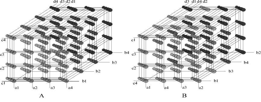
Figure 1. Records in Record Space
B. The Effectiveness of Different Representation
The association rule space S consists of all the possible frequent itemsets. Each possible frequent itemset is a point in this space. If a point in the rule space whose support is greater than support threshold, we call the point a frequent itemset. The objective of the association rule mining in space S is to extract all the frequent itemsets whose confidence is great than confidence threshold.
Comparing with Fig.1, we showed the association rules whose support and confidence values are great than the support threshold 5% and confidence threshold 50% in Fig.2-A. The blue circles are the found rules.
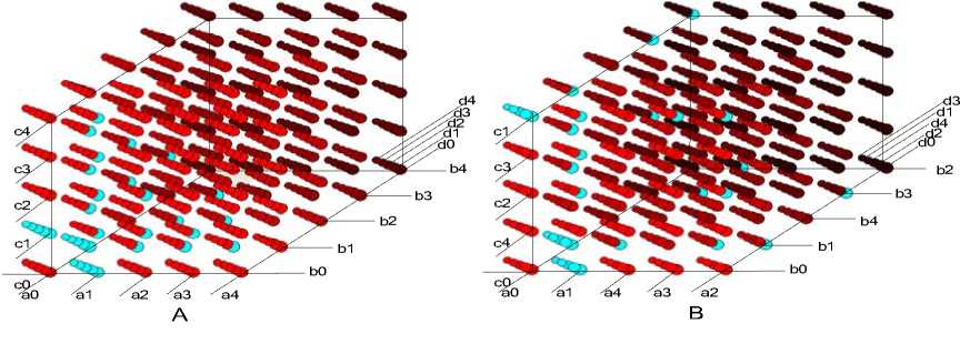
Figure 2. Rules in Rule Space
Comparing with Fig.2-A, after changing the encoding manner, we showed the association rules whose support and confidence values are great than the two thresholds in Fig.2-B. The blue circles are the found rules.
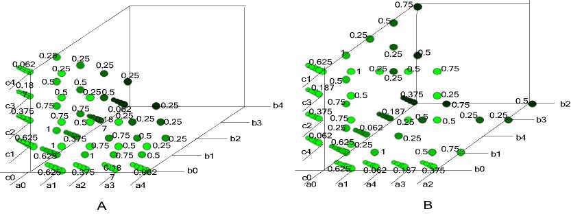
Figure 3. Fitness Values of The Founded Association Rules
In traditional GA, if an appropriate expression manner was chosen and the problem is an easy one to solve, the fitness function should be used to estimate the distance to the nearest global maximum. But if some factors exist in the process which affect the mining greatly or an unsuitable expression was selected, the fitness function will not drive the optimal process effectively. We can see this from Fig.3, A is in an appropriate expression manner and B is in an unsuitable expression manner.
In fact, for a giving dataset D, it is very difficult to decide which representation is a suitable one and at the same time, linkage, deception, epistasis and multimodality always existed in the optimal progress. These will make the traditional GA hard for mining association rules.
-
IV. GROWING EVOLUTIONARY ALGORITHM
A. Growing Evolutionary Algorithm
For building a more accurate classifier, it is very important to find class association rules with larger confidence values. And the mining procedure can be considered as an optimization process in the rule space, in which the CARs can be considered as individuals in a population. The different representations will have a dramatic impaction on how easily the problem will be solved.
Different with traditional EA, we represent individuals with different number of items which can be seen as different age. Every generation was grouped into different groups by age. As the increasing of the age, the support values of the individuals become more and more small. The confidence values were used for selecting good individuals within the same group in which individuals are at the same age. Since the selection was implemented within a limited area (at the same age), it prevents the misleading of the fitness function. A memory set was used in this algorithm to retain the elite ones. When the size of the memory set was set to 1, the algorithm can be used to search the best individual. When the size was set to k, it can be used to find a set of the best individuals.
The proposed growing evolutionary algorithm for data mining is presented below and is illustrated in Fig.1:
Start
I Initialization I
I------Grouping1
' (Ag
Age=1^~ Age=2| ■■■
|Pl,1; Pl 2; Pl,ml| | P2,1; P2 2; .„; P2,m2| I^NjTPn^
groupl | group2| ___________
^Age=N
■—E valuation (on—।
I--------gr^up) 1
[Selection (on group]
jgroupl
| Integrate different groups into one~~|
Crossover
Mutation
-^^Condition
No
Stop)
Figure 4. The Proposed GEA Algorithm
Step 1. Count the support of every item appeared in the given dataset and choose the one whose support value is greater than support thresholds to form the items set I, I={item1, item2, …, itemn}. Randomly initialize a rule population P t , P t =p 1,t +p 2,t +…+p N,t . (t=0). Each rule p i,t (i=1,2,…,N) in it has a class label and several items coming from set I.
Step 2. Select rules in population P t to form different groups, Group n,t . Each rule p n,i,t in the same group has the same age. The age is the number of the items in each rule.
Step 3. Calculate the support value and confidence value of different rules, p n,i,t in different groups.
Step 4. Do selection operator within each group Group n,t , Group n,t+1 = Ts (Group n,t ). The selection operation Ts is defined by the following. (1) Suppress the rules p n,i,t in the group Group n,t whose support value are less than the support threshold “minSupport” and form the group Group’ n,t . (2) Sort the individuals p n,i,t in the group Group’ n,t according to their fitness and choose the first m n highest confidence rules to form the population Group n,t+1 .
Step 5. Integrate the individuals p n,i,t in different group Group n,t+1 into one population P* t+1 , P* t+1 =p* 1,t+1 +p* 2,t+1 +…+p* N,t+1 . Select the best j individuals and put them into the memory set M. Update the memory set, only the best k individuals are remained in it.
Step 6. In population P* t+1 ,, the individual p* n,t+1 reproduces its children p** n,t+1 using an operator of singlepoint random hybridization, Tc. The process of crossover is just like it in conventional The reproduced population is presented with P** t+1.
Step 7. Do a mutation operation. Pt+1=Tm(P**t+1). The mutation operation Tm is defined by the following: (1) Randomly choose an itemi from set I. If there is an itemk in the rule whose attribute is the same with itemi, randomly choose another one until no itemk in the rule whose attribute is the same with itemi. If no such an item can be found, the rule gets its maximal lifetime (the number of items of the rule is equal to the number of attributes of a record) and is deleted. (2) If not be deleted, an itemi is added to it to form a new one.
Step 8. If termination condition is met, stop. The termination condition is that the best individual keep unchanged with continues ten generations. Otherwise, t=t+1; Go step 2.
B. Convergence Analysis
Genetic algorithm can be described as a Markov chain Pt={P(t) , t≥0}. The operations selection, crossover and mutation are independent and stochastic processes. And the new produced generations are related not to the generations before their parents, but to their parent generation.
Definition 1 (Markov chain). A stochastic process {X(n), n≥0} with finite values I={i 0 , i 1 ,… }, is said to discrete time Markov chain or Markov chain if it satisfies the constraint P{X(n+1)= i n+1 | X(0)= i 0 , X(1)= i 1 , … , X(n)=i n }=P{X(n+1)=i n+1 |X(n)=i n }, where P{X(0)= i 0 , X(1)= i 1 ,…, X(n)=i n }>0.
Definition 2 (Transition probability). Probability P{X(n)= j | X(m)=i , n>m} is defined as transition probability of a Markov chain, and is described as Pij(m , n) .
Definition 3 (Satisfying solution set). A solutions set B is said to satisfying solution set, where solutions X(X ∈ B) and Y(Y ∉ B) obey the rule f(X)>f(Y).
Theorem 1. Define P as a transition probability in population space SN, { X ( n )} as a Markov chain, M as global optimum solution, and B as satisfying solutions set.
Let rr
αnB = p{X(n+1)IB =Φ/X(n)IB ≠ Φ} rr
βnB = p{X(n+1)IB = Φ/X(n)IB = Φ}
∞
If ∑(1-βnB)=∞ n =1
lim(αnB)/(1-βnB)=0
n →∞
r
Then lim P { X ( n ) I B ≠ φ } = 1
n →∞
That is to say, if both conditions (5) and (6) are true,
r
{ X ( n )} converges to optimum solutions set M with probability 1. r
Proof P 0( n ) = P { X ( n ) I B ≠ φ } .
According to Bayes formula, we can get
r
P 0( n + 1) = P { X ( n + 1) I B ≠ φ }
= P { X ( n + 1) I B = φ / X ( n ) I B ≠ φ } • { P { X ( n + 1) I B ≠ φ } + P { X r ( n + 1) I B = φ / X r ( n ) I B = φ } • { P { X r ( n + 1) I B = φ }
≦ α nB + β nB P 0 ( n ) (7)
According to (6), we can get
α n B /(1 - β n B ) ≤ ε /2 , where ε >0 and n ≧ N 1
According to (7), we can get
( P 0 ( n + 1) - ε /2) - β nB ( P 0 ( n ) - ε /2)
≦ P 0 ( n + 1) - β nB ( P 0 ( n ) - α nB ≦ 0 ,
Therefore
P 0 ( n + 1) - ε /2 ≤ β nB ( P 0 ( n ) - ε /2)
P 0 ( n + 1) ≤ ε /2 + ∏ n β nB ( P 0 ( n ) - ε /2)
k = 1
n
The condition(5)is equivalent to ∏ βnB = 0,so k=1
∏n βnB ≤ε/2, where n≧N2, k=1
Consequently,
P 0 ( n + 1) ≤ ε , where n ≧ max(N 1 , N 2 )
lim P { X r ( n ) I B = φ } = lim P 0( n ) = 0
n→∞ n→∞ limP{Xr(n)IB≠φ}=1.
n →∞
Theorem 2 For every satisfying solutions set B, if
P { X r ( n + 1) I B = φ / X r ( n ) = X r } ≤ a n
( X r I B ≠ φ )
P { X r ( n + 1) I B = φ / X r ( n ) = X r } ≤ b n
( X r I B = φ )
∑∞ (1 - b n ) =∞ (8)
n = 1
a n /(1 - b n ) → 0 (9)
Then, we can say, { X ( n )} converges to global optimum solutions set M with probability 1.
Proof
α n B = P { X r ( n + 1) I B = φ / X r ( n ) I B = φ )
= P { X r ( n + 1) I B = φ , X r ( n ) I B = φ ) P { X r ( n ) I B = φ }
∑ P { X ( n + 1) I B = φ / X ( n ) = X } P { X ( n ) = X }
X I B ≠ φ
P { X r ( n ) I B = φ
∑ P { X r ( n ) = X r }
≦ a XIB≠φr = a n P{X(n)IB=φ n
In the same way, β n B ≤ b n . With theorem1, we proved it.
Theorem 3 . { X ( n )} converges to global optimum solutions set M with probability 1, when the transition probability of population { X ( n )} obeys the rules like follows,
P{Xr(n+1)IB≠φ/Xr(n)=Xr}=1, where Xr I B ≠ φ (10)
P{Xr(n+1)IB≠φ/Xr(n)=Xr}≥δ, where Xr I B =φ (11)
Proof an=0, bn=1-δ.
According to theorem2, we proved it.
Theorem 4 . The GEA algorithm converges to global optimum solutions set M with probability 1.
Proof.
With the elite strategy in step 5, we can get,
P { X r ( n + 1) I B ≠ φ / X r ( n ) = X r } =1
where Xr I B ≠ φ.(12)
The transition probability is represented as P { T m • T c ⋅ • T s ( X r ) = Y }.
P{Tm•Tc⋅•Ts(Xr)=Y}
∑ P { T m ( X ) = Y } ⋅ P { T c • T s ( X r ) = X } X ∈ S
P{Tc•Ts(Xr)=Xi}
P { T c ( X i , X i ) = X i } ⋅ P { T s ( X r ) = ( X i , X i )}
As can be seen in step6 and 7 , a single-point crossover operator was used. So,
P { T s ( X r ) = ( X i , X i )} = ( f ( X i )/ ∑ N f ( X k ))2 >0
k = 1
P{T c ( X i , X i ) = X i } = 1
P{T c • T s ( X ) = X i } >0
The mutation rate pm(0< pm <1) is greater than 0, therefore,
P{T m ( X ) = Y } >0
P{T m • T c ■ • T s ( X ) = Y } >0
So, p{X(n+1) I в * ф / X(n) = X} > § > о
, where X I B = ф (13)
According to (12), (13) and theorem3, we proved it.
C. Complexity Analysis
Complexity of an algorithm refers to the amount of time and space required to execute the algorithm in the worst case. Determining the performance of a computer program is a difficult task and depends on a number of factors such as the computer being used, the way the data are represented, and how and with which programming language the code is implemented. Here, taking into account the total computational cost and memory requirements, we will present a general evaluation of the complexity of the proposed algorithm.
The time needed to execute it comprises with three main parts:
-
(1) Initialization phase: initialize a population with M individuals. These can be performed in O(M) time.
-
(2) Grouping phase: the time for grouping individuals into different group (group 1 , group 2 , …, group N ) by their ages is O(M). The time for evaluating the fitness of individuals in different group is O(M).
-
(3) Selection, integration, crossover and mutation phase: the time for Ts, Ti, Tc and Tm operation, is O(m 1 2+ m 2 2+…+m N 2), O(M), O(M), and O(M). M is the total numbers of the individuals in the current population, m 1 , m 2 ,…,m N are the individual numbers of different groups, (m 1 +m 2 +…+m N =M).
By summing up the computational time required for each of these phases, it is possible to determine the total computational time of the algorithm. Let the number of global search over iterations is g, hence, the computational time of the whole process is given by
O(M)+O(M X g)+O(M X g)+O((m i2 + m22 +.. .+m N2 ) X g)+O(M X g)+O(M X g)+O(M X g)
=O(M+5 X M X g+(m i 2+ m 22 +^+m N2 ) X g)
=O((5 X M+m i2 + m 22 +^+m N2 ) X g)
It is clear that the computational time of the proposed algorithm is determined by some factors such as population scale M, group scale m i , and the number of global search over iterations.
For a traditional EA, the computational time of the whole process is O((3 X M+M2) X g).
The difference of the two runtimes used by the two algorithms is:
O((5 X M+m 1 2+ m2 2 +^+mN2) X g)-O((3 X M+M2) X g)
=O((2 X M+m i 2+ m 2 2+_+m N2 -M2) X g)
Because of “m 1 +m 2 +…+m N =M”, when M is a large number, the runtime used by traditional EA will greater than the proposed algorithm.
The memory required to run is proportional to the number of individuals M.
-
V. EXPERIMENTS
In this section, we examine how the proposed algorithm can be used to search for association rules. We look on the support value of a rule as the fitness function and on the confidence and support thresholds as constraints. We have conducted an experiment on a 3.0 GHz Pentium PC with 512MB of memory running with Microsoft Windows XP to measure the performance of the proposed approach. The datasets used in the experiment are obtained from the UCI Mache Learning Repository [17].
A. Different Representation
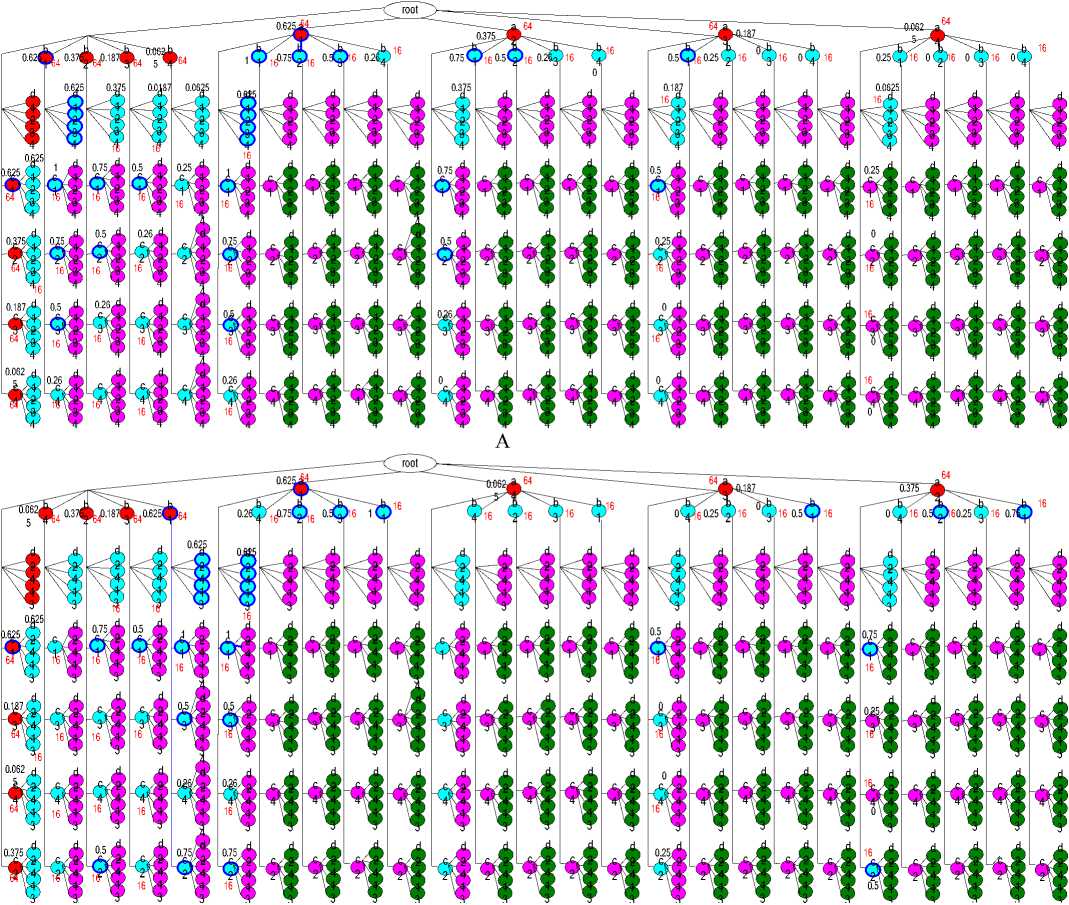
The drawback of the traditional GA used in mining association rule is the inefficiency in dealing with deception, epistasis and multimodality. However, with the proposed algorithm, the affects of these factors were restricted in a certain area in which all the individuals were at the same age. With different encoding manners, the areas of different age are fixed. So the efficiency of the proposed algorithm is independent of representation. We can see that from Fig.5 in which the rules with 1, 2, 3 and 4 items were described by red, pea green, pink and green circle. The rules whose confidence and support values are great than the two thresholds were shown by circle with a blue edge. The founded rules were shown in Fig.4-A, when we represent the individuals in the manner 1. In Fig.4-b, another representation manner was shown. If we look on the number of the circles between two rules as distance, we will find the distance between two rules are fixed with the changing of the encoding manner. However, for a traditional GA, the individuals in one generation were not grouped into different groups. So, the selection operation takes place within the whole generation. And as the changing of the encoding manner, the distance between two individuals of the same generation changed together.
B
Figure 5. The Founded Association Rules in Different Representation Manner
B. The Effectiveness of Different Encoding Manners
In this section, we compared the runtime of the two algorithms GEA and GA when the dataset was coded by different manner. The dataset used is Balance Scale which comes from UCI Machine Learning Repository. There are 625 instances and 3 classes in this dataset. The four attributes are left-weight, left-distance, right-weight and right-distance. We encode the individuals with different encoding manner, which can be seen in talbe.1. In this experiment, we use the two algorithms to find the individual who has the great support value when the confidence of it is greater than confidence threshold. By this examination, we can examine the effectiveness of different encoding manners on the two algorithms. We run the two algorithms ten times separately. Then calculated the mean runtime of the two algorithms and shown them in the table 1.
From the comparison we can see that in the ten different cases, the runtime of the two algorithms for searching the individual with maximal support value are so different. For GA, with different encoding manners, the mean runtime are different. However, for GEA, the mean runtime of the ten implementations are very similar. That is to say, the proposed algorithm GEA is robust with different encoding manner. But, GA is not robust for different encoding manner.
TABLE I. DIFFERENT ENCODING MANNERS
Rep#
Left-Weight Left-Distance Right-Weight Right-Distance Class GA GEA
Name
|
“1” “2” “3” “4” |
“5 ” |
“1” “2” “3” “4” “5” |
“1” “2” “3” “4” “5” |
“1” “2” “3” |
“4” “5” |
“L” |
“B” |
“R” |
Time |
Time |
|
|
Case1 |
001 010011 100 |
10 1 |
001 010011 100 101 |
001 010011 100 101 |
001 010011 |
100 101 |
01 |
10 |
11 |
12.4s |
8.3s |
|
Case2 |
010 001100 011 |
10 1 |
001 010011 100 101 |
001 010011 100 101 |
001 010011 |
100 101 |
01 |
10 |
11 |
16.8s |
8.5s |
|
Case3 |
010 001100 011 |
10 1 |
010 001100 011 101 |
001 010011 100 101 |
001 010011 |
100 101 |
01 |
10 |
11 |
18.0s |
8.6s |
|
Case4 |
010 001100 011 |
10 1 |
010 001100 011 101 |
101 001100 011 010 |
001 010011 |
100 101 |
01 |
10 |
11 |
26.2s |
8.4s |
|
Case5 |
010 001100 011 |
10 1 |
010 001100 011 101 |
101 001100 011 010 |
101 001100 011 010 |
01 |
10 |
11 |
20.6s |
9.1s |
|
|
Case6 |
001 010011 100 |
10 1 |
001 010011 100 101 |
001 010011 100 101 |
001 010011 |
100 101 |
00 |
10 |
01 |
18.5s |
8.8s |
|
Case7 |
010 001100 011 |
10 1 |
001 010011 100 101 |
001 010011 100 101 |
001 010011 |
100 101 |
00 |
10 |
01 |
22.8s |
7.9s |
|
Case8 |
010 001100 011 |
10 1 |
010 001100 011 101 |
001 010011 100 101 |
001 010011 |
100 101 |
00 |
10 |
01 |
34.1s |
9.4s |
|
Case9 |
010 001100 011 |
10 1 |
010 001100 011 101 |
101 001100 011 010 |
001 010011 |
100 101 |
00 |
10 |
01 |
26.2s |
8.3s |
|
Case10 |
010 001100 011 |
10 1 |
010 001100 011 101 |
101 001100 011 010 |
101 001100 011 010 |
00 |
10 |
01 |
15.6s |
8.8s |
|
C. Different Datesets
-
VI. discussion and conlusion
In this section, we compared the two algorithms with different datasets. The results were shown in Table.2, which illustrates the statistic results of computation time, the threshold of confidence and support, the number of instances and attributes of the dataset. When the confidence threshold of dataset Balance Scale was set to 100%, we could almost not find a validated solution. So, we set it to 80%. One important thing we must emphasize is that the complexity of a dataset is decided not only by the number of instances and attributes, but also by the configuration of instances and the number of items and classes in it. So, we should not simply compare computation times between different datasets. From table.2, we can see that the average performance of the proposed algorithm GEA is better than the traditional GA in mining maximal supported association rule.
table ii. C omparision in different dataset
|
Dataset |
Attribute s |
Instances |
Supp(R) |
Conf(R) |
GA(s) |
EA(s) |
|
Balance Scale |
4 |
625 |
>3.8% |
>80% |
12 |
8 |
|
Hayes-Roth |
5 |
132 |
>9.8% |
100% |
2.2 |
2 |
|
Chess |
6 |
28056 |
>0.039% |
100% |
979 |
768 |
|
Car Evaluation |
6 |
1728 |
>33.3% |
100% |
16 |
9 |
|
Nursery |
8 |
12960 |
>33.3% |
100% |
166 |
132 |
|
Contraceptive Method Choice |
9 |
1473 |
>1.4% |
100% |
91 |
69 |
|
tic-tac-toe Endgame |
9 |
958 |
>9.5% |
100% |
59 |
42 |
|
Poker Hand |
11 |
25010 |
>0..56% |
100% |
7296 |
5402 |
|
Adult |
14 |
32561 |
>2.4% |
100% |
2434 |
1844 |
|
Congressional Voting |
16 |
435 |
>50.57% |
100% |
174 |
132 |
The evaluation results have shown that the proposed GEA approach has achieved good performance in comparison with conventional EA algorithms in mining association rules. Being different with GA, the performance of the proposed algorithm is stable with different representations of individuals. This is very useful for dealing problems of linkage and epistasis. Next, we will study on how to pass a message from parent individual to son individuals.
References A Growing Evolutionary Algorithm and Its Application for Data Mining
- J. H. Holland, “Adaptation in natural and artificial systems”, Ann Arbor: University of Michigan Press,1975
- J. H. Holland, “Adaptation progress in theoretical biology”, New York:Academic,vol.4,pp.263–293,1976
- D. E. Goldberg, “ Genetic Algorithms in Search”, Optimization & Machine Learning. 1st ed. New York: Addison-Wesley, 1989
- Albert Orriols-Puig, Jorge Casillas et al., “Fuzzy-UCS: a Michigan-style learning fuzzy-classifier system for supervised learning”. IEEE transactions on evolutionary computation. 13(2),2009.
- D.E.Goldberg.Simple genetic algorithms and the minimal deceptive problem.In L.D.Davis,editor,Genetic Algorithms and Simulated Annealing,Research Notes in Artificial Intelligence,Los Altos,CA,1987.Morgan Kaufmann.
- D.E.Goldberg.Genetic algorithms and Walsh functions:Part II,Deception and its analysis.Complex Systems,3:153–171,1989.
- D.E.Goldberg and M.Rudnick.Schema variance from Walsh-schema transform.Complex Systems,5:265–278,1991
- D.E.Goldberg.Construction of high-order deceptive functions using low-order Walsh coe?cients.Technical Report 90002,Illinois Genetic Algorithms Laboratory, Dept.of General Engineering,University of Illinois,Urbana,IL,1990.
- A. D. Bethke, “Genetic algorithms as funtion optimizers”, Ph.D. thesis, University of Michigan, Ann Arbor, MI.
- D.E.Goldberg, B.Korb, and K.Deb, "Messy genetic algorithms: motivation, analysis, and first results, complex systems, Vol3, pp.493-530, 1989.
- D.E.Goldberg, K.Deb,and D.Thierens, "Toward a better understanding of mixing in genetic algorithm," Journal of the society of Control engineers, Vol.32, No.1, pp.10-16, 1993.
- G. Harik, "Learning linkage to efficiently solve problems of bounded difficulty using genetic algorithms," Doctoral dissertation, university of Illinois at Urbana-Champaign, 1997.
- R. Das, L. D. Whitley, “The only challenging problems are deceptive: global search by solving order-1 hyperplanes.”, Proceedings of the Fourth International Conference on Genetic Algorithms. San Mateo, CA: Morgan Kaufmann, 1991.
- J. J. Grefenstette, “Deception considered harmful”, Pages 75-91 of: Whitley, L. D., Foundations of genetic algorithms, vol.2. San Mateo, CA: Morgan Kaufmann.1993
- T. C. Jones, “Evolutionary Algorithms, fitness landscapes and search.”, Ph.D. thesis, University of New Mexico, Albuquerque, NM.1995.
- R. Agrawal, T. Imielinski and A. Swami. “Mining association rules between sets of items in large databases”. In Proc. of the ACM SIGMOD Conference on Management of Data, Washington, D.C, May 1993.
- D. J. Newman, S. Hettich, C. Blake, and C. Merz, UCI Repository of Machine Learning Databases. Berleley, CA: Dept. Information Comput. Sci., University of California,1998.
