A Hybrid Approach for Real-time Vehicle Monitoring System

In the current digital landscape, computer vision (CV) has seen remarkable advancements, nearing the sophistication levels of human vision. These strides encompass the interpretation of outcomes for basic vision tasks [1, 2]. Previous vehicle detection systems heavily relied on conventional sensing technologies like GPS (Global Positioning System), RFID (Radio Frequency Identification), UWB (Ultra-Wide Band), and BLE (Bluetooth Low Energy) [3, 4]. However, these methods were device-specific and financially burdensome.

Detecting any mobile object within a video holds paramount significance and can be achieved using varied methodologies such as background subtraction (BS), temporal difference, and optical flow [5, 6]. Among these, background subtraction is the most frequently utilized approach to discern different moving objects in video data [7, 8]. This technique leans on a fixed mathematical model that employs a consistent background image, comparing it against each new frame in the video. Background subtraction plays a pivotal role in CV, enabling the identification of mobile objects within video streams without prior knowledge of the frame.

Numerous algorithms have emerged to segregate foreground objects from the background in video sequences [9]. These algorithms find diverse applications across various domains [10, 11]. Presently, many of these algorithms are accessible as web services, such as ChangeDetection.net [12], Stuttgart Artificial Background Subtraction (SABS) dataset [7], and Background Models Challenge (BMC) [13]. These resources hold immense value for researchers and authors, aiding in the processing and comparison of their work against recent contributions.

In the actual scenario, the detection of moving vehicles presents numerous challenges that must be taken into account. This study focuses on analyzing moving vehicles frame by frame and addressing the associated challenges. Fig. 1 illustrates some of our observations during the process of detecting moving vehicles. The first row displays the original images, while the second row shows the adaptation difference for vehicle detection. The evaluation of the results depicted in Fig. 1 is based on the 295th frame (Fig. 1b) out of a total of 421 frames from the video dataset V, = {рх, v2,... v421), which is part of our proposed dataset D.

(a)                                (b)                                (c)

(d)                                   (e)                                    (f)

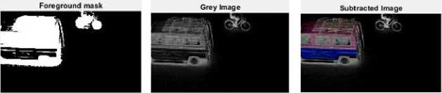
Fig. 1. Moving vehicle detection using an adaptive background. (a) Background, (b) Foreground, (c) Foreground detection, (d) Foreground mask, (e) Gray foreground and (f) Foreground subtraction.

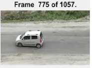
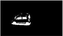
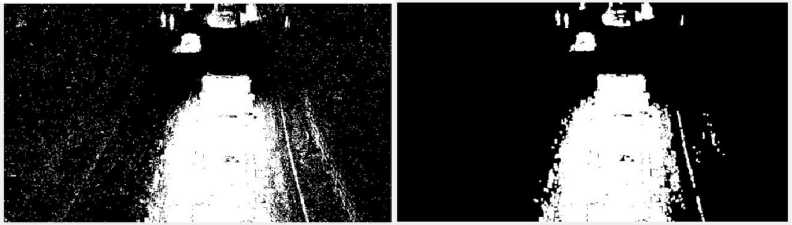
In practice, the background frame (Fig. 1a) is utilized to generate a foreground mask (Fig. 1d) using a threshold value. The vehicles are then detected by employing a median filter-based adaptive background method for background subtraction (Fig. 1f). On the other hand, Fig. 2 demonstrates the application of the frame differencing method for background subtraction on frame v₇₇₅ from a collection of 1057 frames in V j £ D. This particular example represents a challenging cloudy weather condition. As shown in Fig. 2c, the detection bounding box is fragmented into multiple parts or blobs, indicating a suboptimal detection algorithm for such environments. This is primarily attributed to the static threshold used in the algorithm across all images. Such flawed detection can have a significant impact on decision making, which is critical in real-life scenarios.

(a)

Binarized Difference Image

(b)

(c)

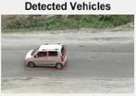
Fig. 2. Moving vehicle detection using a frame difference method for background subtraction. (a) Foreground vehicle, (b) Foreground difference and (c) Detected vehicle.

Due to the COVID-19 pandemic and restrictions on mobility, the general population has been unable to move freely for the past two years. Only essential trips, such as purchasing groceries or visiting pharmacies, have been permitted. In such circumstances, an intelligent traffic surveillance system (ITSS) can play a crucial role by monitoring the movement of vehicles entering highly affected regions. Therefore, the development of an accurate and reliable moving vehicle detector is essential for enabling autonomous operations of vehicles and robots in various environments, both indoors and outdoors. Accurate detection of moving vehicles is particularly important for concepts like driverless cars, especially in challenging environmental conditions. This is because having precise information about the position and velocity of other vehicles is critical for predicting their future movements, which aids in planning the trajectory of the current vehicle. Deep learning (DL) has become widely used for vehicle detection, as demonstrated by recent studies [14, 15].

However, when it comes to real-time deployment in traffic monitoring applications, the computational cost of these methods often poses a limitation. Traditional convolutional neural network (CNN) based object detectors, such as Faster Region-based CNN and RetinaNet, have achieved significant success in natural applications. Nonetheless, their high computational requirements make them unsuitable for running on edge computing units. Additionally, these methods typically require large amounts of training data, which may not always be readily available within a short timeframe for data acquisition and annotation. In a study by Kwan et al. [16], the authors employed the You Only Look Once (YOLO) model to detect and track vehicles under low illumination conditions using low-quality video footage. However, for traffic monitoring applications, high-quality data is preferable to provide better solutions beyond mere detection and tracking, such as vehicle categorization, monitoring vehicle speed, and license plate identification. One challenge with one-stage DL-based methodologies is their limited performance for detecting small objects and their reliance on extensive training datasets. In the field of computer vision, multi-task learning has often been utilized to enhance the overall performance of object detection and semantic segmentation tasks.

In response to the need for a scalable traffic-monitoring system that can be quickly implemented on-board, we have developed a straightforward and efficient framework for image-based lightweight vehicle detection and monitoring. Our solution is capable of real-time operation on Linux-based edge surveillance platforms, and it offers three key contributions.

• •    Firstly, we propose a novel hybrid approach that ensures robust vehicle detection by utilizing background subtraction techniques in diverse environmental conditions. This approach enhances the system's adaptability and reliability.

• •    Secondly, we have designed the algorithm to be lightweight, enabling easy deployment on edge computing devices without compromising real-time performance. Furthermore, the solution includes a simple image analysis component that classifies different types of vehicles, enhancing the real-time user experience.

• •    Lastly, we provide a comprehensive moving vehicle video dataset to the research community, encouraging further exploration in this field. We have rigorously examined our method under various environmental conditions and thoroughly validated its effectiveness, establishing it as the leading choice for vehicle surveillance.

2.    Related Work

• 2.1    Traditional IP Approach

  In recent years, object detection has become a focal point in computer vision (CV) research, with vehicle detection standing out as a crucial area due to its impact on public safety. Reports from July 20211 highlight a significant number of global fatalities annually, largely attributed to fatal accidents, often caused by factors like driver negligence, high speeds, wrong-side driving, malfunctioning indicators, and decreased visibility in adverse weather conditions. The Federal Highway Administration's report from February 20202 underscores that approximately 21% of all yearly road incidents in the United States result from poor visibility during inclement weather [17, 18].

The rest of the paper is divided into the following sections: Section 2 provides an overview of the existing research on vehicle detection. Section 3 describes the proposed architecture, while Section 4 delves into the methodology used and Section 5 showcases the experimental results and compares them with the state-of-the-art (SOTA) approaches. The paper concludes in Section 6.

The field of detecting moving vehicles can be categorized into two distinct research directions: traditional image processing (IP) approaches and DL techniques.

Various techniques have been proposed to achieve accurate vehicle tracking and detection. While the traditional Gaussian mixed model (GMM) [19] has shown promise, it struggles with illumination changes or complex backgrounds. Ji et al. introduced a self-adaptive background approximation and updating algorithm utilizing optical flow theory for traffic monitoring [20].

Their approach involves computing the image difference between current and updated background frames, followed by self-adaptive thresholding based on GMM. Mu et al. adopted a multi-scale edge fusion technique for vehicle detection, integrating differences of Gaussian (DoG) operations [21]. Through the application of various morphological operations, they achieved high accuracy in traffic image analysis. Histograms of Gradients (HOG) [22] and Haar-like features [23] are among the prominent local feature descriptors used in vehicle detection. Machine learning methods, including Support Vector Machines (SVM), Adaboost, and Neural Networks, have also been employed for vehicle detection and classification [22, 17]. While these low-level features offer speed and convenience, they may not comprehensively capture all pertinent information across diverse environments.

Table 1. Related references on vehicle detection in different environments

Methodology	Environment	Accuracy	Year
Gabor-based [25]	Rainy	NILL	2006
Low-level Features [26]	Cloudy, rainy	≈ 94.6% for rainy	2007
TailLight feature (27)	Rainy	≈ 71.0%	2012
Gaussian-based [21]	Cloudy, rainy, foggy	≈ 83.7% for cloudy environment	2016
Associative mechanism [28]	Rainy, foggy	≈ 80.2%	2016
Feature fusion [29]	Rainy, cloudy, misty	≈ 97.7% for misty	2020

Traditional detection methods typically employ two primary approaches: parametric and non-parametric. Nonparametric models segregate foreground and background on a pixel-by-pixel basis, while parametric models aim to construct a background model within the video sequence. Table 1 provides a summary of such related works, and for further details on these methods, [24] is a valuable resource.

• 2.2    DL Approach

  With the increasing popularity of DL, Gan et al. (2019) utilized a teacher-student architecture for the detection and tracking of moving vehicles [30] Similarly, Liu et al. developed a generative adversarial network (GAN) for classifying vehicles in traffic surveillance videos, employing a three-step process [31]. Sang et al. (2018) employed YOLOv2, referred to as YOLOv2_Vehicle, for vehicle detection and utilized six anchors for vehicle model type detection. However, the accuracy of this approach might not always be reliable [32]. Arabi et al. (2020) achieved 90% mean average precision (mAP) for construction vehicle detection using MobileNet. They highlighted the potential application of their approach in safety monitoring, productivity assessments and management [33]. Sri and Rani (2021) improved YOLO by introducing LightYOLO-SPP, a real-time and accurate vehicle detection algorithm based on YOLOv3-tiny. They achieved 52.95% and 77.44% mAP on the MS COCO and PASCAL VOC datasets, respectively, by utilizing the generalized intersection over union (IoU) loss for bounding box regression [34]. Makrigiorgis et al. proposed the AirCam-RTM framework, which combines road segmentation and vehicle detection using unmanned aerial vehicles (UAVs) [35].

3.    Moving Vehicle Detection

• 3.1    GMM-based Approach

• 3.2    Background modelling using GMM

Although these methods perform well when supervised with a sufficient amount of data encompassing different vehicle variants, real-world scenarios involve vehicles with diverse appearances in terms of size, texture, and shape. Consequently, in vehicle monitoring systems, segmentation approaches predominantly rely on appearance-based methods that possess prior knowledge of foreground and background. However, due to the variations in vehicle shapes, there exist several features such as symmetry, edges, and colors that can serve as important cues for detection [36, 25]. While these feature descriptors offer some advantages, they also have limitations. Hence, in this paper, we aim to address these limitations by introducing a hybrid lightweight detector for real-time vehicle monitoring systems.

This paper presents a hybrid approach utilizing machine vision techniques to solve the problem of vehicle detection. Collecting data in real road scenarios can be challenging and demanding, particularly for tasks like vehicle surveillance that involve risks to human life. To address this, we assembled our own vehicle dataset by strategically positioning cameras to minimize occlusions caused by vehicles moving on the left and right sides of the road (refer to Fig. 1 and 2). However, it is important to note that these scenarios are not the only ones considered. Our dataset includes video data captured from high-mounted devices, such as over-bridges and traffic poles, providing top-side views of vehicles in various lighting and geographic conditions (see Table 3). The recorded formats include Joint Photographic Experts Group (JPEG) and Audio Video Interleave (AVI), with a frame rate of 30 frames per second ( fps ).

The main focus of this paper is on vehicle extraction, achieved by processing the video data and making informed decisions. To validate our proposed approach, we conducted experiments under different conditions, including various weather conditions (cloudy and sunny) and lighting conditions (midday and evening). We evaluated several standard SOTA background subtraction methods and determined that the Gaussian Mixture Method (GMM) is the most suitable and robust approach, even under different conditions and in the presence of some level of noise. In the upcoming subsections, we will provide a detailed explanation of our approach and methodology.

Traffic control systems employ surveillance cameras to differentiate between background and foreground moving objects within a given frame of view. To achieve this, one commonly used approach involves the implementation of standard background subtraction methods [37]. Among these methods, the Gaussian Mixture Model (GMM) has proven to be an effective and longstanding solution for addressing challenges in background subtraction [38, 39]. This technique is frequently employed in various applications, such as surveillance, multimedia systems, and optical motion capture devices, to detect moving objects that constitute the foreground within captured video frames [40, 41].

However, determining suitable models for background subtraction without overlooking any moving objects presents its own set of challenges. In certain circumstances, these methods may fail to accurately identify the background, resulting in issues when confronted with factors like variations in illumination or the presence of new objects in the scene that closely resemble the background.

In their study on traffic surveillance systems, Friedman and Russell introduced a model that aims to distinguish different types of background pixels, specifically those related to roads, vehicles, and shadows. To achieve this, they employed a combination of three Gaussian distributions [42]. The Gaussian distributions were assigned labels based on a heuristic approach. The distribution with the highest variance was labelled as “vehicle,” the next one as “road,” and the darkest component as “shadow,” as shown in Fig. 2. It should be noted that this labelling scheme remained consistent throughout the entire process and did not adapt to changes over time.

For the purpose of foreground object detection, each pixel in the surveillance system was compared with each Gaussian distribution. Based on the comparison, the pixel was classified and assigned to the corresponding Gaussian distribution. This process was carried out for every pixel in the image.

The following steps were followed in the proposed model:

• •    Initialization : The three Gaussian distributions representing road, vehicle, and shadow are defined, each with its own set of mean and variance values.

• •    Labelling : The Gaussian distributions are labelled according to their characteristics. The distribution with the highest variance is labelled as "vehicle," the next one as "road," and the darkest component as "shadow."

• •    Foreground Object Detection : For each pixel in the surveillance system, a comparison is made with each of the Gaussian distributions. The pixel is then classified and assigned to the corresponding GMM based on the comparison results.

These steps constitute the basic framework of the model proposed by Friedman and Russell for traffic surveillance systems. However, it's important to note that this model lacks the ability to adapt to changes or deviations over time, as the labelling and Gaussian distributions remain fixed throughout the entire process. The pseudocode is shown in Algorithm 1.

Algorithm 1: An algorithm for GMM background subtraction

• 1:    Input: P i ^ corresponding pixel value

• 2:    Compute: G(p_i) ^ Gaussian correlation for background objects [42]

• 3:    Find best suitable pixel p ^ for the foreground

• 4:    Modify it using Gaussian [42]

• 5:    Pixels not correlated with p_b are considered as connected components

• 3.3    Architecture Modelling

In various real-time applications, such as video conferencing, the camera is typically fixed in position [43]. However, certain applications require the ability to estimate camera motion. To address this need, our algorithm for camera motion estimation involves several essential steps, outlined below in detail:

• •    In this proposed model, the goal is to analyze video sequences by considering a background for each sequence. The video sequences are denoted as a set V , which contains individual video frames V_i = [V 1 , v₂,... vj. Initially, a captured video stream is used, consisting of a number of frames, denoted as i frames.

• •    The model proceeds to the next phase, where it focuses on recognizing the foreground moving objects within each frame. This is achieved by subtracting the background pixels from the current input frame f_i . By performing this, the model isolates the elements that are in motion against the stationary background. However, in order to minimize the impact of noise, a post-processing phase is implemented.

• •    During the post-processing phase, only the frames containing moving objects are considered. These frames are then transformed into a binary image, where the moving objects appear as distinct blobs while the remaining regions are displayed as black. This process can be observed in Fig.1 & 2.

(a)

(b)

Fig. 3. Overview of the proposed detector: (a) followed by (b).

• •    To accomplish this conversion, the model employs various morphological operations. These operations are utilized to selectively segment the objects within the binary image, ultimately merging them into cohesive logical object blobs. This approach is inspired by existing methodologies such as Voigtlaender et al. (2019) and Singh et al. (2015), who have successfully utilized morphological operations to handle similar tasks [44, 45].

• •    Additionally, specific morphological structuring elements are chosen to facilitate the counting of these object blobs. By analyzing the number of blobs, the model is able to determine the frequency and type of objects present within the video sequences.

• 3.4    Functional Requirements

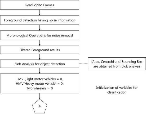
The complete flow of the proposed detector, as illustrated in Fig. 3, starts with the input image. The image is then binarized using the GMM, based on specific features and a threshold. This binary image is further processed to identify and locate the objects of interest. This flow represents the overall procedure followed by the detector to detect the desired objects in an image.

The proposed approach in this paper is defined by a set of functional requirements. These requirements are detailed below:

• •    Capture Video: The system should be capable of capturing videos and storing them in disk(s). The videos serve as the input for extracting successive frames for further processing. The proposed system is designed to work in both online mode, where the input data comes directly from a camera, and offline mode, where the input data is retrieved from saved videos on a hard disk.

• •    Background Extraction: The system should have the ability to separate the background components, denoted as В, from the foreground objects, denoted as F. The background components refer to still objects in the video, while the foreground objects represent moving objects such as vehicles and pedestrians. It is selected based on the entropy criteria of the frame, if it is above the threshold it will update the В.

• •    Vehicle Detection: In order to detect objects, the system utilizes the concept of blobs, which are defined as regions of connected pixels with common properties. The blobs are identified from the foreground objects obtained through the background separation process, using a hybrid approach. The system focuses on detecting vehicles by analyzing and detecting these blobs. Fig. 4 illustrates this process. Blob analysis involves identifying connected regions in the image, where a single blob may contain several connected pixels representing multiple objects or different views of the same object. The detection of blobs is achieved through background subtraction, which identifies the foreground pixels. These pixel blobs correspond to several moving vehicles present in a frame or view. To isolate the blob of a moving vehicle, binarization is performed. The image may contain certain noise, which can be eliminated through simple pre-processing operations. The detected blobs in the foreground images are then utilized to calculate the areas of the vehicle objects. A bounding box is created to localize the detected vehicles, and based on local size features, these vehicles are labelled according to their types.

• •    Counting: Once the vehicle blobs have been identified, a counting algorithm is applied to accurately count and classify the vehicles based on their size or area. The system also maintains a history of the counts throughout the day. It's important to note that, due to privacy concerns, the system does not record the license plates of any vehicles.

4.    Proposed System Overview

• 4.1    Vehicle Detection from Video Streaming

• 4.1.1    Foreground Detection

By fulfilling these functional requirements, the proposed approach aims to capture videos, extract background and foreground components, detect and classify vehicles using blob analysis, and perform accurate counting while respecting privacy considerations.

An overview of our proposed system is depicted in Fig. 3 and in this section we detailed all the modules proposed in this paper.

The process of vehicle detection involves identifying and localizing vehicles that are moving within a given viewframe. This view-frame is typically captured using a static camera that is mounted on poles or over-bridges.

Videos are made up of a sequence of consecutive frames that are related to time. This means that a video can be represented as a function, denoted as f(x, y, t) , where (x,y) refers to the coordinates within the image I at a specific time t.

Static cameras continuously capture images at a certain rate known as fps . These images are then converted into frames for further analysis and processing using IP techniques. Through this process, it becomes possible to analyze the frames and detect the presence of vehicles within them. This is done by identifying features such as the size, shape, and movement of objects within the frames, which are then used to identify and localize the vehicles.

In order to accurately identify the objects in the foreground, a process is followed which begins with the initialization of the background. This involves analyzing a series of images, specifically 150 frames, to gather information about the background and establish a reference for distinguishing between the background and foreground regions continuously.

During this initialization phase, the system calculates an average background representation based on the 150 frames. Among these frames, one specific frame is chosen to serve as the primary background reference, denoted as I_B . This chosen frame acts as a baseline against which the remaining frames are compared.

Each frame is individually compared to the background frame, I_B . If a frame differs significantly in its content from the background frame, it indicates the presence of foreign objects or foreground elements within that frame. In such cases, the foreign object is subtracted from the background frame, effectively isolating the distinct foreground. The resulting subtracted object becomes the representation of the foreground and is denoted as I_F.

By applying this process, the system is able to detect and separate foreground objects from the background, facilitating subsequent analysis and processing tasks specific to the identified foreground elements. The same is described mathematics, below:

Detector = Dect (G, ^, y)                                        (1)

where, G is the number of Gaussian modes which specifies the ability of the model to capture the background. It is always a positive integer value in mixture model, and in the case of this particular task, it is set to be greater than three. Another parameter used is ^ which denotes the initial video frame number that is used to train the background model, denoted by Dect(). For this specific task, the value of ^ is set to be 150.

A threshold value is also used, denoted by y, which is a numeric scalar set to be 0.5. This value is used to determine whether a pixel belongs to the foreground or background region. By optimizing these parameters, the algorithm can minimize the pixel values that are considered for the background region depending on the specific task at hand.

The foreground detector is responsible for comparing each video frame with the background model to determine the existence of individual pixels as foreground or background. The foreground detector then evaluates the foreground mask and detects the foreground objects present in the image captured by the camera. This process is accomplished through the use of background subtraction, which involves subtracting the background model from the video frame to detect the foreground regions. Ultimately, the algorithm's ability to accurately detect foreground objects depends on the effectiveness of these parameters.

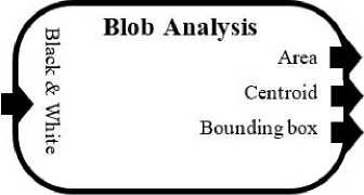
Fig. 4. Overview of blob analysis system

• 4.1.2    Thresholding and Morphological Operation

The subtracted image from the input frame is segmented with the help of threshold value which is practically set for our given task. This segmentation can be performed as:

Dk(x,y) =

1 | Fk(x,y) — Bk — I(x,y) > у

0 |                  otherwise

The equation provided above serves a critical purpose in the segmentation process, which occurs immediately after subtracting the current frame's pixel values from the reference frame's pixel values (v_i+1 — v_i) . This subtraction operation is a key step in detecting moving vehicles within a video sequence. The result of this operation is then passed through a thresholding process. The value of the threshold, denoted by у , is used to compare each pixel value of the frame after subtraction p_i. If p_i is greater than у, it is represented by a '1', and if it is less than у, it is represented by a '0'.

The output of this thresholding process is a segmented image that distinguishes the moving vehicle from the stationary background. The moving vehicle is represented by white pixels, while the stationary background is represented by black pixels. The resulting segmented frame can then be subjected to morphological filters, which are used to remove any noise from the image. These filters can help to improve the accuracy of the vehicle detection algorithm.

Finally, the results of the segmentation process are used as input for the blob analyzer. The blob analyzer identifies and characterizes the individual objects within the segmented image. This process helps to determine the number, size, and position of each vehicle in the video sequence. The overall result is an accurate and reliable detection system that can be used for a variety of applications, such as traffic monitoring or vehicle surveillance.

J = Iopen(I,SE) (3)

where I is the input image, SE is the structuring element and J is the filtered frame.

• 4.1.3    Blob Analysis and Detection

The process of blob analysis involves calculating various statistical measurements for labelled regions within a binary image. This analysis is facilitated by a specific block known as the blob analysis block. This block is designed to generate important information about these labelled sections, including the bounding box, the count of blobs, the centroid coordinates, and the label matrix. A visual representation of these quantities can be observed in Fig. 4.

One notable feature of the blob analysis block is its ability to handle signals of variable sizes for both input and output. This flexibility allows the block to accommodate images of different dimensions and adapt to changing requirements. By supporting variable-sized signals, the blob analysis block enhances its versatility and makes it suitable for a wide range of applications and image processing tasks using vision V library.

E blob    ^ analysis

Once the process of morphological filtering and subsequent segmentation has been applied, the moving object becomes distinctly recognizable in the current frame. As a result, the proposed system generates an output that will be displayed. Upon completing the blob analysis, a bounding box (referred to as BBox) is obtained, specifically outlining the identified object, which in this particular case happens to be a vehicle. In Fig. 5, the bounding box is visually depicted in a vibrant red color, clearly demarcating the area occupied by the vehicle.

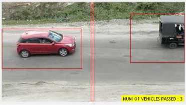
Fig. 5. Detected vehicles in red bounding box

(a)

(b)

Fig. 6. Lines parallel to both the axis

• 4.2    Vehicle Detection and Counting Process

• 4.2.1    Counting Vehicles

• 4.3    Classification of Vehicles via Size

Once the system identifies the presence of a vehicle, the subsequent step involves accurately counting it. This is accomplished by utilizing blob analysis to obtain the centroid of the detected vehicle. The centroid, indicative of the vehicle's center, serves as a reference point for the counting process.

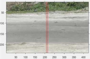
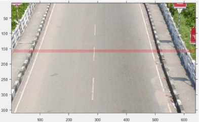
Counting vehicles involves the strategic placement of two parallel lines within the detection area. Whenever, a vehicle traverses these lines, the system increments the count by one. This counting mechanism operates within a designated zone between the parallel lines. Specifically, if the centroid of the detected vehicle falls within this area, the system logs an increase in the vehicle count.

The orientation of the parallel lines is contingent upon the camera setup used for area surveillance. When cameras are predominantly oriented horizontally, the parallel lines are drawn parallel to the X-axis. Conversely, in situations where cameras are vertically oriented, the parallel lines align parallel to the Y-axis. Fig. 6 visually illustrates this counting methodology, adhering to the principle that camera orientation dictates the alignment of the lines – along the X-axis for cameras parallel to the road and along the Y-axis for cameras perpendicular to the road.

The result of performing blob analysis is a set of centroids, which are stored in a matrix of size M x 2. Here, M represents the total number of blobs detected. The matrix has two columns, where the first column corresponds to the x -coordinates of the centroids and the second column corresponds to the y -coordinates of the centroids. Refer to Fig. 7 for a visual representation of this information. The steps can be summarized as: (i) Along the X-axis, x coordinate of the centroid of the blob is checked if it lies in the area between the parallel lines and (ii) Along the Y-axis, the coordinate of the centroid of the blob is checked if it lies in the area between the parallel lines.

One of the challenges in our work is to determine whether the vehicle is heavy or light. This task is achieved with the help of the blob analysis module and is based on the area of the blob that represents the vehicle (refer to Fig. 4). The process involves setting a specific blob size, which is determined experimentally for each type of vehicle, and comparing it to the size of the blobs that cross a set of parallel lines.

In more detail, once the parallel lines are set up, the blob analysis module computes the area of each blob that crosses them. This information is then compared to the specified blob size, and if the blob area is larger than the specified size, the vehicle is classified as heavy. Conversely, if the blob area is smaller than the specified size, the vehicle is classified as light.

To summarize, the classification of vehicles as heavy or light is based on the area of the blob that represents them, and this information is obtained using the blob analysis module and a set of parallel lines. The specific blob size used for each type of vehicle is determined through experimental analysis, and the resulting vehicle blob areas are shown in Fig. 7.

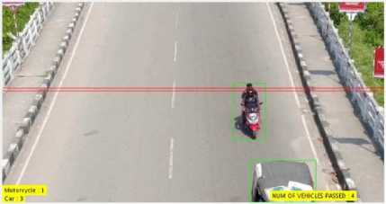
Fig. 7. Classification of vehicles

Table 2. Blob analysis for vehicle type classification

Types	Blob Area ( in pixels )
	Y-axis	X-axis
Two Wheeler / Motorcycle	Т > 2000	Т < 2000
LMV	Т > 2001	Т < 5000
HMV	Т > 5001	Т < 5001

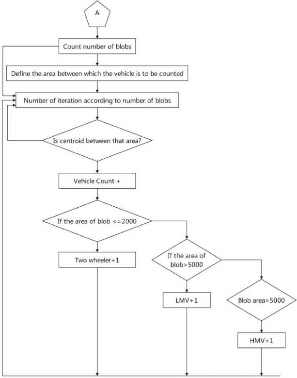
The classification of objects passing through the lines is based on the size of the blob. There are three categories: two wheelers, light moving vehicles (LMVs), and heavy moving vehicles (HMVs), see Table 2. The classification criteria are as follows:

• •    Two Wheelers: If the size of the vehicle blob is less than or equal to T=2000, it will be classified as a two wheeler. This category includes motorcycles, scooters, bicycles, and similar vehicles.

• •    Light Moving Vehicles (LMVs): If the size of the vehicle blob is greater than T=2000 and less than T=5000, it will be classified as a light moving vehicle (LMV). This category typically consists of small cars, compact sedans, and other vehicles of similar size and weight.

• •    Heavy Moving Vehicles (HMVs): If the size of the vehicle blob is greater than T=5000, it will be classified as a heavy moving vehicle (HMV). This category comprises larger vehicles such as trucks, buses, vans, and other vehicles that are generally heavier and larger in size compared to LMVs.

5.    Result and Discussion

By applying these size thresholds, the system can determine the appropriate classification for each blob that passes through the lines. This classification can be useful for various applications, such as traffic monitoring, vehicle counting, or surveillance systems. In order to ensure the accuracy of our vehicle classification, we employ a meticulous process whereby we repeatedly execute the algorithm at multiple intervals while the object of interest, referred to as a "blob," remains within the designated lines. This procedure involves carefully analyzing the captured data to identify and track the blob's position over time. As the blob traverses within the predefined boundaries, we systematically apply the algorithm multiple times, each iteration refining our understanding of the vehicle's characteristics and improving the precision of its classification.

By executing the algorithm repeatedly, we effectively enhance the reliability of our vehicle classification system. This iterative approach enables us to gather a comprehensive set of observations and measurements, allowing for more accurate identification of the vehicle's features, such as its shape, size, and movement patterns.

Table 3. The proposed dataset details

Environment	Dataset D	VideoSize (s)	fps
Cloudy	V 1 = {v 1 > . . . ^ 421 ), V 2 = {v 1 > . . . ^ 1057 1	V 1 = 70.17, Г2 = 176.17	29
Sunny	V 3 = {^ 1 , . . . ^ 76й }, ^ 4 = {^ 1 ,. . . ^ 432 }	Г3 = 128, V4 = 72	29
Night	V 5 = {г 1 , . . . Г 243 }	V5 = 40.5	29

The experiment was conducted on a NVIDIA 1080ti GPU workstation, which is a powerful graphics processing unit designed to perform high-speed parallel processing. The execution of the experiment was carried out using the MATLAB environment, which is a widely used programming language and development environment for technical computing.

To prepare the dataset for the experiment, video data was collected from several different locations with varying lighting conditions. The dataset used in the experiment was carefully selected to reflect the real-world scenarios in which the model is expected to perform optimally.

The results obtained from the experiment are based on the data collected during the optimization of the model. These results are used to describe the performance of the model on video data captured by a stationary camera that was placed on a flyover in Bongaigaon. The video was captured during noon time when the lighting conditions were optimal due to the sun. The specific details of the experiment, including the dataset used and the results obtained, are summarized in Table 3 where fps is frame per second.

• 5.1    Initial Steps on Current Frame

The “current frame” refers to the most recent frame that the system is going to process. In the context of the given information, Fig. 8 displays the current frame, which is numbered as frame 434. This current frame will be compared with the background frame in order to detect and classify vehicles.

The process of comparison involves detecting the foreground in the current frame, which is achieved through segmentation. Once segmentation is complete, the resulting image will be a binary image that requires further processing to filter out noise. The unfiltered binary image will contain a significant amount of noise, as shown in Fig. 9a.

To remove this noise and obtain a more accurate shape of the vehicles, the image will undergo morphological operations. Morphological operations are a set of image processing techniques that involve modifying the shape and structure of an image through the use of mathematical operations. In this case, the unfiltered binary image will be subjected to erosion and dilation. Erosion removes extra pixels while dilation adds pixels to the image, giving it a more accurate shape. The resulting image, as shown in Fig. 9b, will be the filtered binary image, which will be used to detect, count, and classify vehicles in the current frame.

Fig. 8. Classification of vehicles

(a) Segmented image.

Fig. 9. Segmented and filtered frame of the current input frame

(b) Filtered frame

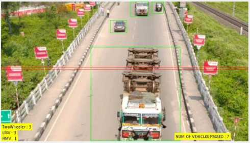
Fig.10. Detection and classification of vehicles

• 5.2    Vehicle Detection & Classification

0.3R+0.59G+0.11B           T

The process of blob analysis is employed on the filtered image to further enhance the vehicle classification, as detailed in Section 4.3 and summarized in Table 2. Blob analysis involves examining distinct regions or clusters of pixels within the image.

By utilizing the centroids of these identified blobs, the system is able to accurately count the number of vehicles present in the scene. Additionally, the system generates bounding boxes around each vehicle, visually represented in Fig. 10. These bounding boxes provide a clear delineation of the vehicles within the frame.

Once the vehicles have been detected and counted, the system proceeds to determine their specific types or categories through a process that relies on the blob area. This information is cross-referenced with the details provided in Table 2, which contains predefined criteria for identifying different types of vehicles.

By utilizing this blob area-based approach and referencing the information in Table 2, the system is able to accurately identify and classify each detected vehicle within the frame.

I_c(x,y, color) ------------> I_{g (ж},_у) ^ = T_bw (x,y) | If T_bw (x,y) >  Т thenT_bw = 1           (5)

Table 4. Comparative analysis of various vehicle detection methods. The values are in percentage

Methodology	DR	FAR	FPR	MOTA
Adaptive Background (AB)	88.76	18.86	82.74	86.75
Frame Differencing (FD)	84.53	24.43	81.33	83.23
GMM	91.86	31.76	90.66	90.85
Hybrid method (proposed)	95.26	35.26	94.26	94.26

• 5.3    Performance Analysis

The performance analysis of vehicle detection methods were evaluated and also detecting the capabilities for moving object detection in terms of detection rate (DR), false alarm rate (FAR), false positive rate (FPR) and Multiple Object Tracking Accuracy (MOTA) are described as follows:

DR = BNTP/(BNTP + BNFN)

FAR = BNFP/(BNTP + BNFP)

FPR = BNFP/(BNFP + BNTN)

where BNTP, BNTN, BNFP and BNFN are the blob based number of true positives, true negatives, false positives and false negatives. DR is a measurement related to the system identifying true positives. FAR is a measurement related to the system correctly identifying the true positives. FPR is a measurement related to the system's correct rejection of false positives. In case of false positive, the proposed method tries to minimise the false alarm.

MOTA = 1 -

S t (m t +f pt +mme t )

^t

MOTA is the accuracy of the tracker in keeping correct correspondences over time, estimating the number of people or objects, recovering tracks, etc . That is to say, it is the sum of all errors made by the tracker over all frames, averaged by the total number of g_t objects and people. Here, m_t , fp_t , and mme_t are the number of misses, of false positives, of mismatches and the number of g_t objects respectively for time t. It is the sum of all errors made by the tracker over all frames, averaged by the total number of g_t objects and people.

In Table 4, we conducted a comprehensive comparison between our hybrid approach and other SOTA methods. The results clearly indicate that our method outperforms the alternatives. Our approach harnesses the strengths of multiple modules, resulting in an impressive accuracy of 95.26% in terms of DR. This accuracy surpasses the second best result achieved by using the GMM alone, exhibiting a significant improvement of 3.4%. Additionally, when considering the MOTA, our method demonstrates a lead of 3.41% over the GMM method and an even more substantial improvement of 7.51% over the adaptive background subtraction method. To ensure a fair comparison, we specifically evaluated a selection of the most advanced handcrafted methods and excluded deep learning methods due to their dependence on large amounts of data and data annotation, which limits their scalability for real-time deployment in industrial settings.

Table 5. Performance measurement of vehicle count and category detection of our hybrid method

Time	12pm (cloud sky, SIDE view)	1pm (clear sky, TOP view)	Inference Cost ( fps )
Total number of vehicles	6	22	20 + 20
Detected	6	20	1.379/40 – 0.0345 ≈ 15.4fps
Missing	0	2
LMV	6	18
HMV	0	2

Time	12pm (cloud sky, TOP view)	1pm (clear sky, SIDE view)	Inference Cost ( fps )
Total number of vehicles	6	22	20 + 20
Detected	6	20	2.597/40 – 0.065 ≈ 15.4fps
Missing	0	2
LMV	6	18
HMV	0	2

Moving on to Table 5, we delve into a qualitative analysis of our proposed approach by focusing on vehicle counting and category detection. This analysis serves as a measure of performance for the approach presented in this paper. It is important to note that the data collected for this analysis was obtained from real-time scenarios with challenging conditions. Table 5 also provides insights into the computational timing complexity of our method, reinforcing its suitability as a real-time solution. The analysis reveals that the inference computational cost of a frame increases proportionally with the number of vehicles present in that frame which in our case turns out to be 15.4 fps , as soon in Table 5.

In our study, we utilized two different figures, namely Fig. 7 and Fig. 10, to demonstrate the method used to calculate the total number of vehicles that cross specific lines. We maintain a record of the history of these lines to keep track of the number of vehicles passing through them. To categorize the vehicles, we utilized a counting algorithm that referred to the thresholds outlined in Table 2.

The counting algorithm segregates the detected vehicle types into three distinct categories. It does so by taking into account the pre-defined thresholds mentioned in the aforementioned table. These thresholds were carefully chosen to ensure that the categorization process was accurate and reliable.

Once the algorithm has identified the vehicles and categorized them, we continuously monitor the blobs until the entire area passes through the line. Only then are the vehicles counted in their respective categories. This ensures that the counting process is precise and that no vehicles are missed or double-counted.

6.    Conclusion

This research paper delves into the challenges associated with the detection, counting, and classification of moving vehicles. The authors explore three distinct approaches: FD, AB, and GMM. Among these methods, FD emerges as a simple yet effective technique, while AB suffers from inefficiency due to internal pixel subtraction. In contrast, GMM stands out as the most robust approach, showcasing superior results. The proposed hybrid vehicle detection method exhibits resilience and weather independence, even in night-time conditions. The study offers a comprehensive analysis of varied vehicle detection techniques aimed at achieving accuracy and robustness. Notably, the vehicle detection rate and MOTA reach 95.26% and 94.26%, respectively, marking a notable improvement of 3.4% and 3.41% over GMM, the second-best approach. Furthermore, the authors intend to extend their proposed method by incorporating a broader range of vehicle types and integrating deep learning principles for enhanced performance.

Acknowledgment

The authors of this paper are thankful to reviewers for their valuable suggestions. Authors are also thankful to Robotics and Computer Vision (RCV) Lab@CIT Kokrajhar for utilizing the NVIDIA GPU server to cover this work.