A Loose Wavelet Nonlinear Regression Neural Network Load Forecasting Model and Error Analysis Based on SPSS

Published Online April 2017 in MECS

Along with the rapid development and improvement of power system, the load forecasting of electrical power has become an independent content in Energy Management System (EMS)[1-3] and it has become an essential part of electric power market transaction management system under the inevitable trend of current power system marketing. In the practical application, the different parts of power system will have different range and accuracy of load forecasting,thus the study on inherent laws and load characteristics of load changing and how to normalize the related factors of load changing in forecasting is of great significance to improve prediction accuracy and load forecasting.

At present, a great deal of theoretical research has been done abroad of the load forecasting of power system, which has reached a high level and some have been put into practical application. China's research on this area starts late, and now has a relatively systematic study. Load forecasting methods can be roughly divided into two categories: a parametric model based approach and a nonparametric model based approach. The principle of the method which based on the parametric model is to analyze the qualitative relationship between the load and the factors which impact the load,build the mathematical model or statistical model of load, such as regression model, time series model, trend extrapolation model and so on. The parameters of these models are obtained by estimating the historical data, and the model is evaluated by the residuals of the model, such as the prediction error[4-6].

Because of the nonlinearity, time variation and the uncertainty of the load forecast, even if the mathematical model can be established, load forecast is also computational complexity, complex structure, difficult to design and implementation and so on.

Application of wavelet analysis theory in the shortterm load forecasting of power system mainly has two aspects[7]. One is the load forecasting using wavelet neural network based on multi-resolution analysis of wavelet series combined with neural network. The wavelet neural networks divide into loose wavelet neural network and compact wavelet neural network. Another is used the combination forecast method, after wavelet quick calculation, decomposition and reply.

Manuscript received October 13, 2016; revised November 18, 2016; accepted December 10, 2016.

No.2006CB303000, No.2007CB316505, corresponding author: Mi Zhang .

• II.    Load Forecasting Based on Loose Wavelet Neural Network

Loose wavelet neural network which is combined with the characteristics of wavelet analysis theory and neural network regard wavelet analysis as preprocessing method of conventional neural network[8-9]. First, decomposing the power load data by wavelet decomposition and get each scale coefficient of the wavelet, then using those coefficients as samples input to the neural network processing. Wavelet analysis and conventional neural network are closely relative but independent each other. Their relationship has shown in Figure 1 as below[10].

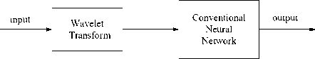
Fig.1. Loose wavelet neural network

• A.    Decomposition forecast reconstruction forecasting model

The Decomposition Forecast Reconstruction loose wavelet neural network is called DFR loose wavelet neural network in which original sequence is generally decomposed by wavelet first, each scale wavelet coefficient is used as input of neural network, and then the prediction value is reconstructed by wavelet. The flow chart has been shown in Figure 2[11].

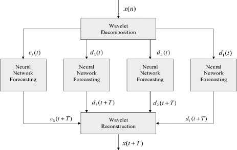
Fig.2. DFR forecasting flow chart

First ， the original sequence is decomposed at t by wavelet decomposition of which scale is j , c represents the low-frequency coefficients sequence in the first j layer at t , d represents the high-frequency coefficients sequence in the first j layer at t . Regard the c and d as the input to neural networks, neural network model being used to forecast for each layer of the wavelet coefficients in order to obtain the predicted value at ( t + T ) , finally these predicted values are used to reconstruct x ( t + T )^[12].

• B.    The selection of the wavelet function

The SNR is the larger the better, and MSE is the smaller the better[6].

N

SNR = 10*log10(Z---^---)(1)

¹=1 ( x - У. ) 2

N

MSE = - E(y, -x, )2(2)

N i = 1

SM =

SNR

MSE

Where y is standard original signal, x is processed estimation signal.

Thus according to the evaluation based on a comparison of SNR and MSE, this paper chooses Db4 as the analysis of the original sequence wavelet function, the two filters of Db4 can decompose the signal into two part: one is a translation by the scaling function as determined by the low-pass section; anther is a translation by the wavelet function as determined by the high-pass section.

• C.    A forecasting based on wavelet coefficients and neural network

The historical load sequence is decomposed by wavelet transform and high and low frequency coefficients are extracted represent different frequencies from each layer is the basic idea of wavelet coefficients and neural networks combined load forecasting[13]. Data in each scale after decomposition are unstable because of the inherent frequency domain aliasing in Mallet algorithm. However, the training of neural networks requires high stability sample data. Thus the threshold is settled to reduce the number of coefficients to extract useful information and remove invalid information. Then, these wavelet coefficients are predicted by the neural network that after threshold effect and normalized. Finally, the forecast daily load values are obtained by inverse wavelet transform. In short, it is to replace the load forecasting to predict the sequence of wavelet coefficients.

The mother wavelet and the size of scale should be selected according to the characteristics of the load. Under some certain prediction requires, selecting the scale too large to improve the prediction accuracy significantly and will reduce the efficiency of computing. In this paper, we selected approximately symmetrical and smooth compactly supported orthogonal wavelet Db4[14] as the mother wavelet, and load data decomposition to 3 scales.

Wavelet decomposition and reconstruction uses a multi-resolution analysis Mallat algorithm. Calculation process is implemented by Matlab language.

Wavelet analysis for load forecasting process can be broken down into the following steps:

• 1)    Decomposition process: A wavelet (Db4) and 3 layers were selected for signal wavelet decomposition.

Mallat decomposition algorithm:

Ao [ f (t)] = f (t)(4)

Aj [ f (t)] = £ H(2t - k)Aj -1[ f (t)](5)

k

Dj [ f (t)] = £ G(2t - k) Aj -1[f (t)](6)

k

In formula (4) 、 (5) and (6), t is the discrete time sequence number, t = 1,2,..., N; f ( t ) is original signal; j is the number of the layers, j = 1,2,..., J , H , G are the wavelet decomposition filter in the time domain, actually are filter coefficients; wavelet coefficients of the approximately part (low-frequency part) of signal f ( t ) at j -layer is A ; wavelet coefficients of the details part (high-frequency part) of signal f ( t ) at j -layer is D . The results obtained are shown in Figure 3.

CD1 wavelet coefficients

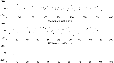
Fig.3. Db4 3 layers for signal wavelet decomposition

The contents of Mallat decomposition algorithm is: Assumed A is detected by the discrete signal f ( t ) .The approximately part of signal f ( t ) at j -layer is obtained by point sampling interval through the results of convolution which are wavelet coefficients A of low-frequency which is obtained by the convolution of wavelet coefficients A _y_₁ of the approximately part at j - 1 -layer and decomposition filter G . The signal f ( t ) will be broken down into two parts through decomposing by Mallat algorithm. One is wavelet coefficients A of low-frequency at low-frequency sub-band, another is wavelet coefficients D of the details part at high-frequency sub-band^[15].

• 2)    Threshold was selected for coefficients of each layer after decomposition, details coefficients for soft threshold; due to frequency domain aliasing in the wavelet coefficients obtained by Mallat decomposition algorithm, data in each scale after decomposition are unstable. However, the training of neural networks requires high stability sample data. Thus the threshold was settled to reduce the number of coefficients to extract useful information and remove invalid information.

In practical engineering applications, for nonlinear signal wavelet decomposition, the same threshold was used in each of the scales apparently inappropriate and removes useful information in the lower scales. Therefore, hierarchical threshold was considered to solve this problem. According to characteristics of historical load sequence and results of actual simulation, the following conclusions can be obtained.

Select thresholds for decomposed wavelet coefficients of each layer. No thresholds for low-frequency parts and the corresponding threshold were selected according to their characteristics for high-frequency part.

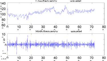
Fig.4. Wavelet coefficients obtained by wavelet decomposition for the original load

By subdivision of the high-frequency part we can obtain:

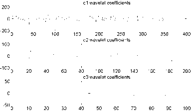
Fig.5. High frequency (details) parts of the decomposition coefficients of different scales

• 3)    Wavelet coefficients processing: in order to avoid saturation phenomenon in neurons of neural network, the training data samples for normalizing to guarantee the input data located in[0,1] . The formula for normalizing is as follow:

'

min     max    min

Then, to predict the values of each layer which are normalized by neural networks respectively.

Bring into the self regression neural network to predict. In the input layer with the following formula retranslated back coefficient.

'

max    min        min

Among formula (7) and (8),  L' represents the value normalized, L represents wavelet coefficients, Lmax、 L represent the maximum and the minimum of wavelet coefficients of each layer respectively.

Reconstruction process: wavelet coefficients which processed by the neural network can obtain load value of prediction date through the wavelet reconstruction algorithm. Reconstruction algorithm is as follows:

A j [ f ( t )] = 2[ ^ h ( t - 2 k ) A j + f ( t ) + E g ( t — 2 k ) D j + f ( t )] ^ kk

Where j is the number of layers of decomposing; h 、 g are wavelet reconstruction filters in the time domain which are actually filter coefficients.

Reconstruction algorithm    content[15]:    wavelet coefficients of the approximately part of signal f (t) at 2 j -scale ( j -layer) is A which is the sum of two convolutions. One is A which is the approximately part of signal f (t) at 2j+1-scale ( j +1-layer) after interval point zero insertion and reconstruction filter h . Another is Dj+1 which is the details part of signal f (t) at 2 j+1-scale ( j +1 -layer) after interval point zero insertion and reconstruction filter g . This process is repeated until 20 -scale and get the reconstructed signal.

• III.    Example Verification

  In this paper, the load data of Yichang, Hubei Province, China was adopted as the experiment data from September 1, to September 30, 2005. (24 points per day, 720 points totally.) The load sequence with three-scale was decomposed by Mallat algorithm and forecasting^[16].

• A. Single-sample T-test analysis for the original load data based on SPSS software

SPSS is one of the world’s common statistical packages, applies not only to the social sciences, but also applies to economics, medicine, psychology, etc[16]. Compared with other international authoritative software, its most notable feature is no programming, completed with menus and dialog mode of operation, easy to learn and easy to operate.

• 1.    The purpose of the single-sample T-test

• 2.    The basic steps of single-sample T-test

The purpose of the single-sample T-test is the sample data from a general being used, and deducing if there is any significant difference between the overall mean and the developed test value. It is the overall mean of hypothesis testing.

• 1)    Proposed the original hypothesis

The original hypothesis H of single-sample T-test: there is no difference between the overall mean and the developed test value, expressed as H_o : u = u ₀ . u is the overall mean, u is the developed test value.

• 2)    Selected the test statistic

When the overall distribution is normal N ( u , 5 ²) , Sampling distribution of the sample mean is still normal. The mean of normal distribution is u , the variance is

• ₂ 5 5

5 / n . In X : N(u,—) , u represents the mean of n normal distribution, when the original hypothesis was established that u = u0; 52 is the overall variance, n is the total number of samples. When the overall distribution subject to normal distribution approximately, the overall variance is unknown generally, at this point the sample variance S 2 was used to replace it, thus the test statistic obtained for statistic as:

t =

X — u

Where the statistic obedience to the distribution which degrees of freedom is t .The test statistic of the singlesample t is t test statistic. When the original assumptions holds, replace u with u .

• 3)    The observed value of the test statistic and probability value P was calculated

The purpose of this step is to test the observed value of the test statistic and the corresponding probabilities. The sample means, the sample variance and the total numbers of samples were substituted into formula (10) by SPSS software automatically^[17], and then the observed value of the test statistic and probability value ^P was being calculated.

• 4)    Given significance level, and make decisions

If the probability value ^P less than the significance level ^a , the original hypothesis is rejected, think there is a significant difference between the overall mean and overall test values. On the contrary, if the probability value P greater than the significance level ^a , the original hypothesis is accepted, think there is no significant difference between the overall mean and overall test values.

Table 1. Data sample statistics

Single-sample statistics
	N	Mean	Std. Deviation	Std. Error Mean
Sept.1	24	674.8125	28.86922	5.89290

Table 2. Data sample test

Single-sample test
	Test value = 674.8
	t	df	Sig.(2-tailed)	Mean Difference	95% Confidence Interval of the Difference
					Lower	Upper
Sept.1	.002	23	.998	.01250	-12.1779	12.2029

Table 1 shows the average value from September 1 Yichang of electricity load is 674.8125MW, the standard S deviation is 28.86922, and the mean standard error (    )

n is 5.89290. In Table 2, the observation of t statistic is 0.002, df shows the degrees of freedom is 23, two-tailed probability value of t statistic observed value is 0.998, 95% confidence interval of the overall mean is (674.812.1779，674.8+12.2029). Two-tailed test is to compare α and P , given α 0.05, due to P = 0.098 greater than 0.05, accept the original hypothesis thinking that there is no significant difference between the overall mean and overall test values.

Test load data from September 2 to September 30 similarly and finishing as the following Table 3.

Table 3. Load data sample statistics from September 2 to September 30

Single-sample statistics
	N	Mean	Std. Deviation	Std. Error Mean
Sept.2	24	677.5000	22.83441	4.66106
Sept.3	24	649.9833	22.23674	4.53906
Sept.4	24	608.2458	44.74958	9.13447
Sept.5	24	651.0375	27.85899	5.68669
Sept.6	24	637.8167	37.98541	7.75374
Sept.7	24	628.7625	51.19076	10.44927
Sept.8	24	695.7125	23.86920	4.87228
Sept.9	24	708.9083	20.46095	4.17657
Sept.10	24	734.3958	22.20630	4.53284
Sept.11	24	729.0875	26.19976	5.34800
Sept.12	24	735.5875	25.86986	5.28066
Sept.13	24	784.2875	31.91617	6.51486
Sept.14	24	815.3125	25.90510	5.28786
Sept.15	24	810.6917	32.29612	6.59242
Sept.16	24	846.1375	31.55670	6.44148
Sept.17	24	741.7792	32.41905	6.61751
Sept.18	24	724.4500	22.51786	4.59644
Sept.19	24	756.8958	38.64488	7.88835
Sept.20	24	830.2875	52.10123	10.63512
Sept.21	24	772.3667	57.28148	11.69253
Sept.22	24	722.7458	26.07638	5.32282
Sept.23	24	748.5167	28.38866	5.79481
Sept.24	24	769.4417	30.46799	6.21925
Sept.25	24	757.8042	25.21843	5.14769
Sept.26	24	760.7083	23.44676	4.78605
Sept.27	24	772.1583	19.45537	3.97131
Sept.28	24	767.2417	21.21607	4.33071
Sept.29	24	783.0417	31.87878	6.50723
Sept.30	24	797.5833	23.92598	4.88387

As can be seen from the Table 3, the standard deviation and the standard error of the mean of load data of September 30-day is small, indicating that data is changed slightly, and there is no significant difference between the data and the mean.

• IV.    Forecasting Results

• A.    Comparison of the original load signal and the predicted value

We input the command in command window of Matlab and we can get the graph of the comparison of the reconstructed signal and the original and the graph of error between the predicted value and the actual value, as they are shown in Figure 6 and Figure 7 as follows:

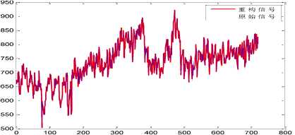
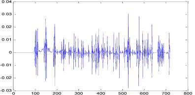
Fig.7. The graph of error between the predicted value and the actual value

The graph of the original signal and the reconstruct signal are quietly match which can be seen in the above figure, and absolute value of the error is less than 3% which proves the wavelet neural networks in the area of power system load forecasting turns out good results.

• B.    Error analysis based on SPSS software and Wilcoxon signed rank test

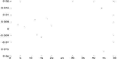
In Figure 8, the horizontal axis is the time point, 48 points in total; the vertical axis represents the percentage error. We can see that the error range is [ - 2%,2%] , providing a high prediction accuracy.

The basic idea of Wilcoxon sign rank test methods:

first, calculate on the difference between the sample observations, arrange according to their absolute value, excluding the samples that difference is zero, smallest class is one and so on. If there is some equals between the absolute value of the differences in the order sequence, the difference between the averaged values as these rank. Then restore the original sign, sum the rank of the sign respectively, T ⁺ represents the sum of positive rank, T ^- represents the sum of negative rank. Select one of the smaller rank and as a statistic. But Wilcoxon sign rank test in SPSS is just a simple operation.

We choose SPSS software to test the differences between the two related samples. The predicted and actual values of September 30 were tested; the result is shown in Figure 9 as follows.

Hypothesis Test Summary

Null Hypothesis

The median of differences between predicted and actual equals 0.

Test

Sig.

Decision

Related-Samples Wilcoxon Sign Rank Test

0.030

Reject the null hypothesis.

Asymptotic significances are displayed. The significance level is .05.

Fig.9. Hypothesis testing summary

The chart in Figure 9 shows that the significance level is 0.05, asymptotic significant is 0.030 less than 0.05(given α 0.05) which is enough to illustrate the error between the predicted value and the actual value is small.

• V.    Conclusion

Based on the investigation of multi-resolution analysis methods of wavelet transform, load sequence is analyzed using Daubechies (N) wavelet series[9]. By analysis and comparison, ultimately determine that the most suitable wavelet function for load data in this paper is Db4. Through the multi-resolution analysis of power system load sequence to determine the wavelet decomposition level of the time sequence, to achieve the multi-resolution analysis of small samples in the power system load sequence.

The method of DFR power system load sequence wavelet neural network forecasting was given first. Decomposing the load data by wavelet to obtain wavelet coefficients, then wavelet coefficients are brought into the neural network to predict, reconstruct the predict value by wavelet to get the final forecast load data. This load forecasting method combines wavelet analysis of good temporal localization features and good neural network nonlinear approximation ability.

SPSS software was selected to analyze the original data and error. Testing the differences between the two related samples, and we got the asymptotic significant is 0.030 less than 0.05(given α 0.05) shows that there is no significant difference between the predicted value and the actual value. It has better prediction accuracy.