A mathematical model to develop a nomadic livestock connection with industrial objects

In Mongolia, nomadic livestock has been developed and practiced since ancient times. Currently, more than 90% of nomadic livestock is still traditional. Nowadays, the expansion of urban areas, the extraction and production of mining resources are intensifying in our country. This is having a negative impact on our traditional livestock farming. In particular, the development of nomadic husbandry in accordance with current needs and requirements is a priority.

Therefore, we will formulate mathematical models based on an ecological-economic model [1] and will be executed qualitative analysis. Due to intensive mining and other industries, the environment is polluted. In [1] , the problem of keeping the pollution level at a certain level by devoting an amount of funds to environmental protection was studied. However, the level of pollution is a very general concept, and the interests of industrial enterprises that directly benefits from nature are always affected by conduct production on the territory where it exists. For this reason, in order to maintain the natural balance at a certain level, let’s the amount of investment for natural restoration or protection the industrial object’s is K 2 (t), and the ecological capacity of the livestock enterprise is S ( t ) . Also let’s the production volume of the industrial object is Y ( t ) . Then the following balance equation can be written:

S ( t ) = — m • Y(t) + h • K 2 (t)                     (1)

Here, m is the constant that indicate how intensively the production has a negative impact on nature and h is the constant that benefit of natural protection work.

Using (1) equation, we formulate the mathematical model of livestock enterprises and industrial objects, and the analysis of their optimal equilibrium ratio points and the research results of determining the optimal land ratio are presented in the following sections.

• 1    Model of nomadic livestock enterprises and industrial ob jects

  1.1    Model of Industrial objects

The amount of Y(t) is represented by the Cobb-Douglas production function:

Y (t)= A • K ^a (t) • L ^1-a (t), (0 1)               (2)

In (2) , let the size of main fund of the industry be K i (t) and the amount of fund devoted to nature restoration be K 2 ( t ) .

It is assumed that u 1 and u 2 of the produced products are used to increase the amount of funds for production and nature protection, respectively. Therefore, the mathematical model of the long-term profitable operation of the industrial object is formulated in following equation [1] , [2] , [4] , :

T lim 1 [ (1 — ui(t) — U2(t)} • YTt)dt ^ max

T →∞ T J                     L(t)

K 1 ( t ) = U 1 (t)Y(t) - ^K 1 (t)

K 2 (t) = U 2 (t)Y(t) - ^K 2 (t)

^L(t) = g • ^{L ( t )}

S(t) = — mY (t)+ hK 2 (t)

0 <  u 1 (t) <  1 , 0 <  u ₂ (t) <  1 , u 1 (t) + u ₂ (t) <  1

Here, g >  0 is the growth coefficient of L(t) workforce, ^ is the loss coefficient of main fund, S(t) is the grazing area assigned to the livestock enterprise. But u 1 (t)Y(t) and u ₂ (t)Y(t) are the amount of investment for industry production and nature protection or restoration. Then

0 <  1 — u 1 (t) - u ₂ (t) <  1

is the percentage of funds for consumption and

[1 - u 1 ^{( t )} - u 2 ^{( t )}] • L(t)

is an indicator of average consumption per person.

In above model, the boundary conditions are not specifically written because we study the optimal versions of the equilibrium ratio that keeps K i (t), K 2 (t), S(t) at a constant level. Due to we use the long-term profitable production represented by the functional (3) .

In the model (3) , (4) :

Kin - Ki(t) Кin - K2(t) K(t) = Lt ’ K(t) = W these conversions are done, it will be changed to the following form:

T lim - / (1

T →∞ T

— u 1 ( t ) — u 2 ( t )

• AK ^a dt ^ max

K(t)= u i (t)AK ^a - t + g)K(t)

Kit) = U 2 AK ^a - (ц + g)K(t)

S(f) = ( - mAK ^a (t) + hK(t)^L(t) 0 <  u 1 (t) <  1 , 0 <  u ₂ (t) <  1 , u 1 (t) + u ₂ (t) <  1

1.2    Livestock enterprise model

We let N be the number of animals, S(t) be the size of grazing area, and y(t) be the density of grass per unit area, then the model can be written by formula (7) - (8) . Therefore, the model [2] [3] of long-term profitable operation of the livestock enterprise is:

T lim —  p(t)Ndt ^ max

T →∞ T

N

^{y ( t )} = g⁽y^{( t ))} - F⁽y^{( t ))} •

S ^{( t )}

p(t) = aF (y(t)) - bp ^Y (t), (0 <  1)

Here, a is the metabolism coefficient, b is the energy loss factor, and γ is the basic exchange rate, particularly, y = 4 is derived based on statistical analysis in [5] [6] . g(y) is the plant regeneration function satisfying the conditions that g(0) = g(y) = 0 , g"(y) <  0 . Also F(y) is a function representing the amount of grass eaten by one animal that meets the conditions

F (0) = 0 , F'(y) >  0 , F"yy) <  0 , lim Fyy) = F <  от .

y→∞ and p(t) is the average weight of the animal. A connection of two models (5) - (6) and (7) - (8) is shown by the following scheme in Fig. 1.

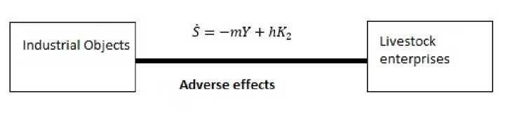
Fig. 1. Scheme of the model

• 2    Analysis of optimal equilibrium ratio points

Let K ( t ) = const, S(t) = const in (5) — (6) , y(t) = const, p ( t ) = const in (7) — (8) , the model turns to the following maximization problem:

(1 — u1 — u2)AKa ^ max(9)

u 1 AK ^a — nK = 0 , n = № + g

K = mAKa ^ K • (u—h — n) =0

hm

0 <  u i <  1 , 0 <  u ₂ <  1 , u 1 + u ₂ <  1

p(t) • N ^ max

g(y) — f (y) • NN = 0

aF (y) — bp ^Y = 0

From equation (10) , U2 = П— — is obtained. So П^^ — < 1 .

• a)    If П ^^m = 1 , it will be impossible to carry out production as K = K i = 0 , all capital is devoted to nature protection or restoration.

• b)    Consider the case u i + U 2 <  1 , U 2 = П—— <  1 . In this case, tion can be profitable. Also

  produc-

  
  

u = n • k ^1-a ,  K = ^AK ^a

1A               h and the objective function is formulated as follows

(1 — n i — П 2 ) A

α u 1 A  ^1-α

-

η

u 1

-

η · m h

-α

· η ^1-α

· u ₁ ¹

α

-α

.

Therefore, we have to consider the following maximization problem:

M ( u ₁ ) = (1 — u ₁ —

η · m ^α 1     _- α

· u ^1-α · A ^1-α · η ^1-α h ¹

^ max

0 <  u i <  1 —

η · m h

An optimal solution exists of above problem and it is found:

M 0 ( u i ) = 0 ^ — u.- a +(1 — u i — n-m ) • -A-      =0 ^ u i = a ( 1 — nm ) .

h 1 — a                   h nJ

And from equation (11) ,

p(t) = ( a ) ^Y • F ¹ (^y), N = S • FP^ b'                        F (y)

is found and the objective function is formulated by

Np(t) = S • ( a ) ^Y • F(y) • g(y)

Therefore, it is necessary to consider the following maximization problem:

L( ^y ) = ( a ) ^y • f ~-Y (y • g(y) ^ ^max

The maximum point of the function L(y) is to the right of maximum point g(y) function’s. Because

1 - Y

----> 0 ^ g ( y ) = 0 ^ y op G L(y).

γ and g'(yop) < 0. Now let’s study the stability of system equations (11) for stationary points (yop,pop). For this, we write the Jacobian matrix:

'g (Pop) - F^Ур) • NN 0   \ a • F'Уро)      -bypo-1)

and the characteristic equation is

A 2 — ^{( g ( y} pp} - ^{F , y} Pop) • “FT

S

-

N bypO-1)a - (g (yop) - F (yop) • -^yp^1 = 0 S and its solution is x     g'(Ppp)— F’yoo) • N — bypop1 ± VD

X1,2 =--------------------2-------------------- g'(Pop) — F'РУор) • NN — bypp-1 ± g'(Pop) — F'Pypp) • NN + bypO-1

and

N

A 1 = g (P op) ^— F (P op) — <  0 ,   X 2 = — byp Op ¹ <  ⁰

S here,

D=

N ²

g (P op) ^— F (P op ) •    ^— byp Oo- ¹

S

+ ⁴ g^P op ) ^— F ' (P op ) • — byp Op ¹ .

S

Therefore, the system is stable and (y _op ,p _op ) becomes the stabilization point. We summarize the above results and write the following corollary.

Corollary 2.1. Long-term steady-state points for both two models in (5) (8) are

K i = (unA) 1-^a • L ⁽⁰⁾ e gt , K 2 = K 2 ⁽⁰⁾ • e ( - ^^t ,         P op )

and optimal control is

u * = u 1 + u ₂ = ⁿ m (1 — a ) + a.

h

Also, the optimal adjustment of the unit area is made by the equation:

N op    ^{g ( y} op' ⁾

S = F^) .

• 3    The case where the industrial ob ject requires land

The previous sections included the negative impact that industry objects and the amount of products it produces is reduce the grazing area of livestock enterprises. But we did not include in detail the case of demand another grazing area. To consider this case, suppose that the amount of products it produces depends on three main factors: the grazing area S 1 , the main fund for production K 1 , and the labor force or population L 1 . Then

Y(S i ,K i ,L i ) = As e K a L -a 0 <  a,e <  1 .

It provides the definition of the production function. Let be the number of people working at the livestock enterprise is L 2 and be the total area between the industrial object and the livestock enterprise is S _max . Then S = S max — S i . Here, S is the area per livestock enterprises.

If we consider both the industrial object and the livestock enterprise as a monolithic system operating on its own area and set a long-term profitable operation goal, we can write the following objective function. Where lim 1 ( TT(1 — u(t) — u2(t)) • Y^dt + Л p^dt) ^ max (12) t^^ T0O v '        2’ Li(t)      0O L2(t) ’             1 ’

If we initially assume that Li(t) = const, L2(t) = const, S(t) = const and Si(t) = const, each increment of functional (12) take to the maximum value from the research in section 2 when -^- < 1. That maximum value is obtained as follows op        ηm op ηm ui = a(1 —    ), u2 = -^.

and optimal values of grass density y ^op are found. In other words, for the constants S and S 1 , whose sum is S _max , each increment of the functional (12) takes its maximum value in the following case:

2α-1

(1 - u o" - u o") • A i^a • n 1- a • ( u ^ p )      • S _i ^1-a +

+ ( S max — S 1 ) • ^ a ^ ^Y • g^L^ • ( F ( y on ) ) ^{1 - 1} .

If we use the notation as

1      -α2

11 — ui" — u^j • A 1-a • n 1-a • (ui") 1-a = Ci > 0, a! y • gyo • (f (yop)) y-i=c2 > o, bL following optimization problem can be set. It includes:

β

M ( S i ) = C i • S^ + (S max — S i ) • C 2 ^ max

⁰ <  S i <  S max

In here if i — a >  1 or i — a <  1 , either the industrial object or the livestock enterprise is not needed when

C i • ( S i op ) 1^ + (S max

β

— S O" ) • C 2 <  max( S max • C 2 ,C i • S m - x ) .

But when а + в <  1 and

C i • ( S Op ) 1^ + (S max

-

β

S Op ) • C 2 >  max( S _moI • C 2 , C i • S mJ )

the conditions are met, the optimal follows

solution for the area is obtained as

S O" = I¹/

C 2 - 1

C i )

1-α

-

α-β .

Conclusion

In the first section of this work, we formulated of the mathematical models of the production ob ject and the livestock enterprise located in a limited area, and the balance equation (1) expressing the connection between these two objects was newly formulated. In this regard, some conditions of the mathematical model were formulated. Also, we analyzed the points of an optimal equilibrium ratio of the models (5)-(6),(7)-(8), and the stable state points for the long-term existence of the two objects were found. In this regard, we found the optimal control of the model. As well as, we formulated the corollary. In section 3, the mathematical formulation of the proper amount of the area in two objects is presented.