A model to assess the risk of bankruptcy for agricultural firms in Krasnoyarsk region

The global financial crisis and as a consequence the instability in financial markets have caused a drastic increase in the number of firms going out of business on the background of the overall economic downturn. In this context, an early recognition of pending problems is important for ensuring continuity of one’s business. In connection to this there is a necessity to work out an effective model to assess the risk of bankruptcy, which would allow to predict potential distress situations in Russian companies. The purpose of the present work is to construct such a model of bankruptcy risk assessment for agricultural firms of Krasnoyarsk region.

The structure of the model consists of a number of consecutive steps:

Step 1. To select a set of significant financial ratios for further analysis, to define classes of financial condition, put together linguistic characteristics.

Step 2. To reduce the dimensionality of the selected set of factors by applying the method of principal component analysis and to construct factors hierarchy.

Step 3. To derive discriminant functions for the principal components having been identified in the second step mentioned above.

Step 4. To produce an aggregate matrix for level recognizing on a standard 01-qualifier.

Step 5. To perform hierarchy nodes convolution and assign the firm to one of the classes defined in Step 1 mentioned above.

During the first step, we define three groups of firms as follows: financially sound (Class 3), financially unstable (Class 2), and financially distressed (Class 1) firms. Next we create a set of data containing twenty three various financial indicators, such as profitability ratios, solvency indicators, and business activity indicators, which describe different aspects of financial standing of the agricultural firms [1]. The model was constructed according to data for 2006, 2007. Model check was made according to data for 2008.

Let us define the so-called linguistic variable, “Factor level” [2], with the term set of L to have the form:

L = {Low level ( L ), Average level ( A ),

High level ( H )},                   (1)

Next we introduce F 0 as a criterion of financial soundness and solvency. The linguistic variable provides a qualitative description of the firm’s condition related to F 0 . We set the following meaning for the linguistic characteristics:

• –    low F 0 means the firm is in a critical financial condition and falls into Class 1 enterprises;

• –    average F ₀ means the firm is financially unstable and fits into Class 2 enterprises;

• –    high F 0 means the enterprise is financially sound and qualifies for Class 1 enterprises.

If the company relates to financially distressed enterprises it indicates a high risk for bankruptcy. Likewise. Financially unstable firms have an average risk for default and financially sound enterprises indicate a low risk for bankruptcy.

The second step is to identify the factors based on factor analysis (after a preliminary analysis for multicollinearity). These factors give the largest contribution into dispersion of the resultant indicator F₀ , which describes a probability of bankruptcy through linguistic characteristics. The algorithm of factor analysis can be found in [2].

The following financial ratios are incorporated in the factor analysis:

Factor 1 – k 1 – inventory coverage ratio; k 2 – circulating assets in fill rate; k 3 – economic efficiency of operating assets; k 4 – a part of working capital in circulating assets; k 5 – a part of fill rate in operating assets.

The first factor includes indicators showing how effectively the firm manages its assets and inventories. Current assets coverage indicator can be adduced as a short characteristic; k 7 – financial dependence index; k8 – equity flexibility ratio; k 9 – payback term for equity of the investment.

Factor 2 includes indicators which characterize the use of the firm equity capital.

Factor 3 – k 10 – equity capital ratio; k 11 – loan capital ratio, k 12 – return of assets pricing; k 13 – common production profitability.

The third factor measures profitability of the firm derived from equity and loan capital indicators. It denotes a profitability factor.

Factor 4 – k 14 – cash ratio; k 15 – quick ratio; k 16 – current ratio; and k 17 – return on production assets.

The factor incorporates indicators of liquidity and the earning capacity of the production, therefore it can be called a solvency indicator.

To define the significance of the factors, let us consider tab. 1.

Table 1

Total Dispersion

Factors	Initial Eigenvalues
	Total	Variance (П), %	Cumulative, %
1	6.676	29.026	29.026
2	4.006	17.417	46.444
3	3.178	13.818	60.261
4	1.833	7.967	68.229

Let the sign « » » denotes the indifference between two factors, i.e. the two factors are equally significant, and the sign « ^ » denotes the preference of one factor to another, i.e. one of the factors is more significant than the other for the root element of the hierarchy ( F 0 ). The set of symbols and factors forms a system of relative preference. In this case this system looks as follows:

Ф = { F i ^ F 2 = F 3 ^ F 4 }. (2)

It is based on the results of factor analysis. Relative contribution of individual factors to the total dispersion of characteristics [3] is compared:

Fi } Fi+1 if Пi > Пi+1 is more than on 10 % and Fi ≈ Fi+1 if Пi> Пi+1 is less than 10 %, where Пi is the percentage of dispersion due to a particular individual factor (i. e. the contribution of that factor to the total dispersion), the subscript i denoting the factor number (thus П1 is the percentage of dispersion due to the first factor).

Let us build a tree-like hierarchy of the given factors (fig. 1).

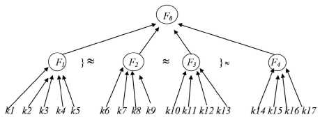
Fig. 1. Tree-like hierarchy of factors

In our case being based on system (2) and the Fishburn method [3] we have the following weights 3111

• (    8, 4,4,8) for factors F ₁, F ₂, F ₃, F ₄, accordingly.

Now we have to categorize the firm belonging to classes mentioned above using each factor

(F1,F2,F3,F4). We attempt to assign the firm to one of the three groups of financial viability by using each factor, based on the indicators selected as described above. This will be the third step in developing the model. Using the indicators determining each factor we reciprocate the functions with the best predictive ability. In this work it is a linear discriminant function. To reciprocate this function (3)–(6), we perform a discriminant analysis (tab. 2). In accordance with its results we have the following functions:

F 1 =- 0.14 ■ k 1 - 1.055 ■ k 2 + 0.441 - k 3 + + 1.534 ■ k 4 - 1.667 ■ k 5 + 2.462,

F ₂ =- 0.713 ■ k 6 + 0.738 ■ k 7 -- 0.88 ■ k 8 + 1.658 ■ k 9 - 0.08,

F₃ =- 0.063 ■ k 10 - 0.139 ■ k 11 + + 0.912 ■ k 12 + 2.044 ■ k 13 + 0.802, F ₄ = 0.071 ■ k 14 - 0.008 ■ k 15 + + 0.462 ■ k 16 + 3.339 ■ k 17 - 1.014.

According to the correlation index (> 0.5 for all factors) we can that correlation is satisfactory. Significance p is less than 0.001 for all functions, which implies that the mean values of each of the functions are significantly different for various classes. High eigenvalues (more than one) indicate a good (appropriate) choice of discriminant functions (tab. 3).

Let us calculate the average value between the centroids for the functions of factors and we can establish the intervals of the firms belonging to each class (tab. 4).

Table 2

Statistical calculations for discriminant functions

Function	Eigen value	Variance, %	Cumulative, %	Canonical Correlation	Wilks’ Lambda	Chi-square	Sig. p
F 1	1.431	94.8	94.8	0.767	0.382	32.758	.000
F 2	3.316	95.6	95.6	0.877	0.201	55.403	.000
F 3	2.022	89.9	89.9	0.818	0.269	45.249	.000
F 4	3.463	96.7	96.7	0.881	0.200	55.467	.000

Table 3

Group Centroids Functions

Group	Function in Group Centroids
	F 1	F 2	F 3	F 4
Class 3	1.409	2.324	1.856	2.641
Class 2	.333	–2.211	.014	–.725
Class 1	–1.286	–.223	–1.402	–1.482

Table 4

Intervals of belonging in accordance with discriminant functions of factors

Value range	Parameter level	Risk of bankruptcy by each of the factors
For F 1 :
F < - 0.4765	Class 1	High
- 0.4765 <  F <  0.871	Class 2	Average
0.871 <  F	Class 3	Low
For F 2 :
- 1.217 <  F 2 <  1.0505	Class 1	High
F 2 <- 1.217	Class 2	Average
1.0505 <  F 2	Class 3	Low
For F 3 :
F 3 < - 0.694	Class 1	High
- 0.694 <  F 3 <  0.935	Class 2	Average
0.935 <  F 3	Class 3	Low
For F 4 :
F 4 <- 1.1035	Class 1	High
- 1,1035 <  F 4 <  0,958	Class 2	Average
0.958 <  F 1	Class 3	Low

Having established the intervals of firm belonging to each class and having calculated the functions for their quantitative estimation we can make a convolution using the hierarchy stages. For the linguistic variable “Factor level” with the L term-set given by (1) and the hierarchy of factors we use the conventional three-level 01-classifier (SFC) [3] which acts as a group of functions of the firm class belonging, where these functions are trapezoidal triangular numbers (fig. 2):

trapezoidal numbers SFC; M is the belonging matrix, у is the belonging of the firm to one of the classes by means of each particular factor (3)–(6). For example if by F ₁ (3) the enterprise belongs to Class 1, the element y _x1 is equal to 1 while the rest of the elements in the first line are zero. The same principle applies to other lines of the matrix.

Let us compare the estimated value with the tabular data and evaluate a probability of bankruptcy in terms of linguistic characteristic ( tab. 5 ).

0 1 ( x ) = <

5(0.4 - x ),0.2 <  x <  0.4

0 1 ( X ) = <

5( x - 0.2), 0.2 <  x <  0.4

1,0.4 <  x <  0.6

5(0.8 - x ), 0.6 <  x <  0.8

0 з ^{( x} ) = *

' 0,0 <  x <  0,6

5( x - 0.6), 0.6 <  x <  0.8

Let it be that F₀ = x , and x = a 01-carrier in (6) (the [0,1] segment of real line).

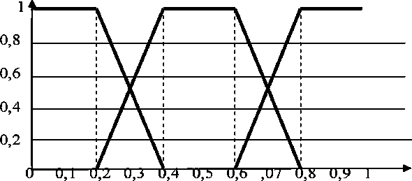
Fig. 2. System of trapezoidal belonging functions on the 01-carrier

The standard classifier projects the fuzzy linguistic variable onto the 01-carrier, and does so in a consistent manner, producing a pattern of symmetrically distributed classification stages (0.1; 0.5; 0.9). In these stages, the value of one particular membership function is equal to 1 (one) while all other functions are zero. The analyst’s uncertainty about correctness of classification decreases or increases linearly with the distance from the stages, the sum of membership functions being equal to 1 (one) in all points across the carrier.

We find F 0 by means of matrix convolution:

'Y11    Y12 Y13' ' 0.1 ^ F, = pmv = (p> p2...Pn)• .. vY1 n    Y 2 n * . Ymn у • 0.5 V 0.9 у , the coefficient vector of the factors

where P is

(3111);

8, 4,4,8

' 0.1'

0.5

_v 0.9 _у

is the vector of vertices of

Table 5

SFC-based classification of the level of F ₀

F 0 limit	Parameter level	Degree of evaluation certainty (membership function), magnitude ∙100 %
0 <  F0 <  0.2	Low	1
0.2 <  F 0 <  0.4	Low	P 1 = 5 • (0.4 - F 0 )
	Average	1 -0 1 =0 2
0.4 <  F 0 <  0.6	Average	1
0.6 <  F 0 <  0.8	Average	0 2 = 5 • (0.8 - F 0 )
	High	1 -0 2 =0 3
0.8 <  F 0 <  1	High	1

The final result is a linguistic description of the degree of probability of bankruptcy as well as the degree of the analyst’s certainty as to the correctness of recognition. Therefore the conclusion about the risk degree not only has a linguistic form but also contains a characteristic of the assertions quality.

All in all we have finished the development of the model for assessing the risk of firm default. Let us illustrate the model by evaluating the factors for the agricultural firm GPKK “Borodinskoye”, Rybinsky Region. While this company was included into the group of financially unstable enterprises, its data were not used in the developing of the model. In our calculations we use formula (2) and the data from tab. 6.

According to (3)–(6) we have: F 1 = –0,5 – Class 1; F 2 = –1,6 – Class 2; F 3 = –0,22 – Class 2; F 4 = –0,32 – Class 2;

F ₀ = PMV =

f t

4 4 8 )

V 0

0.5 = 0.35.

According to tab. 5 the company belongs to Class 1 with the probability 5 (0.4–0.35) = 0,25 and to Class 2 with the probability 1–0.25 = 0.75. The company does not have sufficient coverage for floating assets and fill rate (by factor F 1 = –. 05 it falls into Class 1), the company’s equity is inefficient, and it exhibits low profitability and solvency indicators (by factors F 1 , F 3 , and F 4 it belongs to Class 2). The risk of bankruptcy in the nearest perspective is assessed as average.

Table 6

Balance Sheet Data

Item	Thousand roubles	Item	Thousand roubles	Item	Thousand roubles	Item	Thousand roubles
Earnings	16 028	Inventory	12 552	Balance value	36 937	Long-term liabilities	2 023
Cost price	17 686	Long-term receivables	1 967	Charter capital	100	Loans and credits	6298
Profit before tax	–1 658	Short-term receivables	514	Added capital	45 606	Accounts payable	36 110
Fixed assets	20 132	Cash	100	Net profit	–53 200	Current liabilities	42 408
Noncirculating assets	20 132	Floating assets	16 508	Capital and reserves	–7 494	Liabilities	36 937

Based on financial information provided by Agricultural Agency of Krasnoyarsk region, we have calculated the value of F 0 for ten different agricultural firms in each of the classes and compared the results with their initial classification. Full matching (i. e. when probability = 1) of our findings and conclusions with the original classification was 82.5 %. We observed any case when after the analysis a company originally classified as a financially distressed class 1was transferred to Class 3 (financially stable firms). It proves that the model is adequate and appropriate for assessing the risk of bankruptcy.

In addition to conventional methods, the proposed model of bankruptcy risk assessment can be an effective tool in evaluating financial position of a company, that can enable company’s management to continuously monitor the financial situation in the company for the risk of default. It is never late to mitigate the risks with the development of a package of measures particular important in the unstable conditions of economic environment [4–6].