A Modified Particle Swarm Optimization Technique for Economic Load Dispatch with Valve-Point Effect

Автор: Hardiansyah

Журнал: International Journal of Intelligent Systems and Applications(IJISA) @ijisa

Статья в выпуске: 7 vol.5, 2013 года.

Бесплатный доступ

This paper presents a new approach for solution of the economic load dispatch (ELD) problem with valve-point effect using a modified particle swarm optimization (MPSO) technique. The practical ELD problems have non-smooth cost function with equality and inequality constraints, which make the problem of finding the global optimum difficult when using any mathematical approaches. In this paper, a modified particle swarm optimization (MPSO) mechanism is proposed to deal with the equality and inequality constraints in the ELD problems through the application of Gaussian and Cauchy probability distributions. The MPSO approach introduces new diversification and intensification strategy into the particles thus preventing PSO algorithm from premature convergence. To demonstrate the effectiveness of the proposed approach, the numerical studies have been performed for three different test systems, i.e. six, thirteen and forty generating unit systems, respectively. The results shows that performance of the proposed approach reveal the efficiently and robustness when compared results of other optimization algorithms reported in literature.

Еще

Particle Swarm Optimization, Economic Load Dispatch, Non-Smooth Cost Functions, Valve-Point Effect

Короткий адрес: https://sciup.org/15010441

IDR: 15010441

Текст статьи A Modified Particle Swarm Optimization Technique for Economic Load Dispatch with Valve-Point Effect

Published Online June 2013 in MECS

Most of power system optimization problems including economic load dispatch (ELD) which have complex and nonlinear characteristics with heavy equality and inequality constraints. The objective of the ELD of electric power generation is to schedule the committed generating unit outputs so as to meet the required load demand at minimum operating cost while satisfying all unit and system equality and inequality constraints. Several classical optimization techniques such as lambda iteration method, gradient method, Newton’s method, linear programming, Interior point method and dynamic programming have been used to solve the basic economic dispatch problem [1]. These mathematical methods require incremental or marginal fuel cost curves which should be monotonically increasing to find global optimal solution. In reality, however, the input-output characteristics of generating units are non-convex due to valve-point loadings and multi-fuel effects, etc. Also there are various practical limitations in operation and control such as ramp rate limits and prohibited operating zones, etc. Therefore, the practical ELD problem is represented as a non-convex optimization problem with equality and inequality constraints, which cannot be solved by the traditional mathematical methods. Dynamic programming method [2] can solve such types of problems, but it suffers from so-called the curse of dimensionality. Over the past few decades, as an alternative to the conventional mathematical approaches, many salient methods have been developed for ELD problem such as genetic algorithm [3, 4], improved tabu search [5], simulated annealing [6], neural network [7, 8], evolutionary programming [9]-[11], and particle swarm optimization [14]-[17].

Recently, Kennedy and Eberhart suggested a particle swarm optimization (PSO) based on the analogy of swarm of bird and school of fish. In PSO, each individual makes its decision based on its own experience together with other individual’s experiences [12]. The individual particles are drawn stochastically towards the position of present velocity of each individual, their own previous best performance, and the best previous performance of their neighbors. It was developed through simulation of a simplified social system, and has been found to be robust in solving continuous non-linear optimization problems [13]. The main advantages of the PSO algorithm are summarized as: simple concept, easy implementation, and computational efficiency when compared with mathematical algorithm and other heuristic optimization techniques.

In this paper, a novel approach is proposed to solve the non-smooth ELD problem with valve-point effect using a MPSO technique. The application of Gaussian and Cauchy probability distributions into the PSO is a useful strategy to ensure convergence of the particle swarm algorithm. Feasibility of the proposed MPSO method has been demonstrated on three different test systems, i.e. six, thirteen, and forty generating unit systems. The results obtained with the proposed method were analyzed and compared other optimization results reported in literature.

II. Economic Load Dispatch Formulation

2.1 Economic Load Dispatch (ELD) Problem

The objective of an ELD problem is to find the optimal combination of power generations that minimizes the total generation cost while satisfying equality and inequality constraints. The fuel cost curve for any unit is assumed to be approximated by segments of quadratic functions of the active power output of the generator. For a given power system network, the problem may be described as optimization (minimization) of total fuel cost as defined by (1) under a set of operating constraints.

Ft =Z F (Pi) = ZkP 2 + bipi + Ci) i=1 i=1 (1)

Where ^T is total fuel cost of generation in the system ($/hr), a_i , b_i , and c_i are the cost coefficient of the i th generator, P_i is the power generated by the i th unit and n is the number of generators.

The total generation cost is minimized subjected to the following constraints:

Power balance constraint,

Generation capacity constraint,

Pd =Z Pi - Plos.

i = 1

where Pi, min and Pi, max are the minimum and maximum power output of the i th unit, respectively. PD is the total load demand and PLoss is total transmission losses. The transmission losses PLoss can be calculated by using B matrix technique and is defined by (4) as, nnn

p, = У У pb p + У b.p + b^
2.2 ELD Problem Considering Valve-Point Effects

Loss i ij j 0i i00

i=1 j=1

where B ij is coefficient of transmission losses.

For more rational and precise modeling of fuel cost function, the above expression of cost function is to be modified suitably. The generating units with multivalve steam turbines exhibit a greater variation in the fuel-cost functions [15]. The valve opening process of multi-valve steam turbines produces a ripple-like effect in the heat rate curve of the generators. These “valvepoint effects” are illustrated in Fig. 1.

The significance of this effect is that the actual cost curve function of a large steam plant is not continuous but more important it is non-linear. The valve-point effects are taken into consideration in the ELD problem by superimposing the basic quadratic fuel-cost characteristics with the rectified sinusoid component as follows:

F t = E F ( P )

i = 1

=z i=1

aP + bP + C + _v| e , ^x sin ( f. ^X ( ^P ,m,n

P i

where F_T is total fuel cost of generation in ($/hr) including valve point loading, e_i , f_i are fuel cost coefficients of the i th generating unit reflecting valvepoint effects.

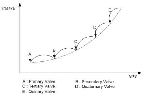
Fig. 1: Valve-point effect

III. Particle Swarm Optimization

3.1 Overview of Particle Swarm Optimization

The PSO method was introduced in 1995 by Kennedy and Eberhart [12]. The method is motivated by social behaviour of organisms such as fish schooling and bird flocking. PSO provides a population-based search procedure in which individuals called particles change their position with time. In a PSO system, particles fly around in a multi dimensional search space. During flight each particles adjust its position according its own experience and the experience of the neighboring particles, making use of the best position encountered by itself and its neighbors.

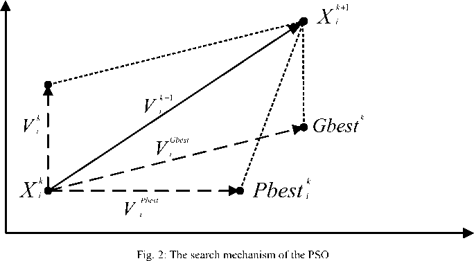
In the multidimensional space where the optimal solution is sought, each particle in the swarm is moved toward the optimal point by adding a velocity with its position. The velocity of a particle is influenced by three components, namely, inertial, cognitive, and social. The inertial component simulates the inertial behavior of the bird to fly in the previous direction. The cognitive component models the memory of the bird about its previous best position, and the social component models the memory of the bird about the best position among the particles. The particles move around the multi-dimensional search space until they find the optimal solution. The modified velocity of each agent can be calculated using the current velocity and the distance from Pbest and Gbest as given below.

W = W max

where,

( (W max

min

Iter max

x Iter

V^k + 1

W X Vk + C X r X (Pbestk - X)+ C2 Xr x(Gbestk -X)

WW max , min

initial and final weights

Iter

max

maximum iteration number

Iter

current iteration number

where,

V i^k

velocity of individual i at iteration k

X i^k

position of individual i at iteration k inertia weight

The approach using (7) is called “inertia weight approach (IWA)”. Using the above equation, a certain velocity, which gradually gets close to Pbest and Gbest can be calculated. The current position (searching point in the solution space), each individual moves from the current position to the next one by the modified velocity in (6) using the following equation:

xk+1

= x k + V k + 1

C 1 , C 2

acceleration coefficients

where,

Pbest k

best position of individual i at iteration k

Gbestk

x i ⁺ ¹

k+1

current position of individual i at iteration

best position of the group until iteration k

r1,r2

V ^k + 1

random numbers between 0 and 1

velocity of individual i at iteration k+1

In this velocity updating process, the acceleration coefficients C 1 , C 2 and the inertia weight W are predefined and r 1 , r 2 are uniformly generated random numbers in the range of [0, 1]. In general, the inertia weight W is set according to the following equation [13]:

Fig. 2 shows the concept of the searching mechanism of PSO using the modified velocity and position of individual based on (6) and (8) if the value of W, C 1 , C₂, r₁, and r₂ are 1.

The process of implementing the PSO is as follows:

Step 1: Create an initial population of individual with random positions and velocity within the solution space.

Step 2: For each individual, calculate the value of the fitness function.

Step 3: Compare the fitness of each individual with each Pbest. If the current solution is better than its Pbest, then replace its Pbest by the current solution.

Step 4: Compare the fitness of all individual with Gbes t. If the fitness of any individual is better than Gbest , then replace Gbest .

Step 5: Update the velocity and position of all individual according to (6) and (8).

Step 6: Repeat steps 2-5 until a criterion is met.

3.2 Modified Particle Swarm Optimization

Coelho and Krohling [18] proposed the use of truncated Gaussian and Cauchy probability distribution to generate random numbers for the velocity updating equation of PSO. In this paper, new approaches to PSO are proposed which are based on Gaussian probability distribution ( Gd ) and Cauchy probability distribution ( Cd ). In this new approach, random numbers are generated using Gaussian probability function and/or Cauchy probability function in the interval [0, 1].

The Gaussian distribution ( Gd ), also called normal distribution is an important family of continuous probability distributions. Each member of the family may be defined by two parameters, location and scale: the mean and the variance respectively. A standard normal distribution has zero mean and variance of one. Hence importance of the Gaussian distribution is due in part to the central limit theorem. Since a standard Gaussian distribution has zero mean and variance of value one, it helps in a faster convergence for local search.

Here the Cauchy distribution Cd , is used to generate random numbers in the interval [0, 1], in the social part and Gaussian distribution Gd , is used to generate random numbers in the interval [0, 1] in the cognitive part. The modified velocity equation (6) is given by

' WV + C G ()( Pbest i - X ) "

■ C 2 C d ()( Gbest^k - X ) ,

K =

2 - ф - ^ф ² - 4 ф

where Ф = C i ⁺ ^C 2 , Ф > 4 .

The convergence characteristic of the system can be controlled by ^ф . In the constriction factor approach (CFA), ^ф must be greater than 4.0 to guarantee stability. However, as ^ф increases, the constriction factor K decreases and diversification is reduced, yielding slower response. Typically, when the constriction factor is used, ^ф is set to 4.1 (i.e. C 1 , C ₂ = 2.05) and the constant multiplier K is thus 0.729.

IV. Results and Discussion

To verify the feasibility of the proposed method, three different power systems were tested: (1) 6-unit system with valve-point effects and transmission losses, (2) 13-unit system with valve-point effects and transmission losses are neglected and (3) 40-unit system with valve-point effects and transmission losses are neglected.

Test Case 1: 6-unit system

The system consists of six thermal generating units with valve point effects. The total load demand on the system is 1263 MW. The parameters of all thermal units are presented in Table 1 [14], followed by coefficient matrix B_i j losses.

The obtained results for the 6-unit system using the MPSO method are given in Table 2 and the results are compared with other methods reported in literature, including GA, PSO, PSO-LRS, NPSO, and NPSO-LRS [19]. It can be observed that MPSO can get total generation cost of 15,441 ($/hr) and power losses of 12.216 (MW), which is the best solution among all the methods. Note that the outputs of the generators are all within the generator’s permissible output limit.

Test Case 2: 13-unit system

This system consists of 13 generating units and the input data of 13-generator system are given in Table 3 [10]. In order to validate the proposed MPSO method, it is tested with 13-unit system having non-convex solution spaces. The 13-unit system consists of thirteen generators with valve-point loading effects and have a total load demands of 1800 MW and 2520 MW, respectively.

The best fuel cost result obtained from proposed MPSO and other optimization algorithms are compared in Table 4 and Table 5 for load demands of 1800 MW and 2520 MW, respectively. In Table 4, generation outputs and corresponding cost obtained by the proposed MPSO are compared with those of DEC-SQP, NN-EPSO, and EP-EPSO [20]. The proposed MPSO provide better solution (total generation cost of 17517.0118 $/hr) than other methods while satisfying the system constraints. In Table 5, generation outputs and corresponding cost obtained by the proposed MPSO are compared with those of GA-SA, EP-SQP, and PSO-SQP [20].

The proposed MPSO provide better solution (total generation cost of 24019.8924 $/hr) than other methods while satisfying the system constraints. We have also observed that the solutions by MPSO always are satisfied with the equality and inequality constraints by using the proposed constraint-handling approach.

Test Case 3: 40-unit system

This system consisting of 40 generating units and the input data for 40-generator system is given in Table 6 [10]. The total demand is set to 10,500 MW.

The obtained results for the 40-unit system using the MPSO method are given in Table 7 and the results are compared with other methods reported in literature, including PSO, PPSO, and APPSO [21]. It can be observed that MPSO can get total generation cost of 121,649.20 $/hr, which is the best solution among all the methods. These results show that the proposed methods are feasible and indeed capable of acquiring better solution.

The optimal dispatches of the generators are listed in Table 7. Also note that all generators’ outputs are within its permissible limits.

Table 1: Generating units capacity and coefficients (6-units)

Unit	min ⁱ (MW)	max ⁱ (MW)	a	b	c	e	f
1	100	500	0.0070	7.0	240	300	0.035
2	50	200	0.0095	10.0	200	200	0.042
3	80	300	0.0090	8.5	220	200	0.042
4	50	150	0.0090	11.0	200	150	0.063
5	50	200	0.0080	10.5	220	150	0.063
6	50	120	0.0075	12.0	190	150	0.063

0.0017 0 . 0012 0.0007 - 0.0001 - 0.0005 - 0.0002

0.0012 0 . 0014 0.0009 0.0001 -0.0006 -0.0001

0.0007 0 . 0009 0.0031 0.0000 -0.0010 -0.0006

B j =

- 0.0001 0 . 0001 0.0000 0.0024 -0.0006 - 0.0008

- 0.0005 -0 . 0006 -0.0010 -0.0006 0.0129 -0.0002

_- 0.0002 -0 . 0001 -0.0006 -0.0008 -0.0002 0.0150 _

BOi = 1.0e-3 *[- 0.3908 - 0.1297 0.7047 0.0591 0.2161 - 0.6635]Boo = 0.0056

Table 2: Comparison of the best results of each methods (P D = 1263 MW)

Unit Output	GA	PSO	PSO-LRS	NPSO	NPSO-LRS	MPSO
P1 (MW)	474.8066	447.4970	447.4440	447.4734	446.9600	447.1874
P2 (MW)	178.6363	173.3221	173.3430	173.1012	173.3944	173.5060
P3 (MW)	262.2089	263.0594	263.3646	262.6804	262.3436	260.9553
P4 (MW)	134.2826	139.0594	139.1279	139.4156	139.5120	144.0583
P5 (MW)	151.9039	165.4761	165.5076	165.3002	164.7089	163.2156
P6 (MW)	74.1812	87.1280	87.1698	87.9761	89.0162	86.2934
Total power output (MW)	1276.03	1276.01	1275.95	1275.95	1275.94	1275.216
Total generation cost ($/hr)	15,459	15,450	15,450	15,450	15,450	15,441
Power losses (MW)	13.0217	12.9584	12.9571	12.9470	12.9361	12.2160

Table 3: Generating units capacity and coefficients (13-units)

Unit	P min (MW)	P max (MW)	a	b	c	e	f
1	0	680	0.00028	8.10	550	300	0.035
2	0	360	0.00056	8.10	309	200	0.042
3	0	360	0.00056	8.10	307	200	0.042
4	60	180	0.00324	7.74	240	150	0.063
5	60	180	0.00324	7.74	240	150	0.063
6	60	180	0.00324	7.74	240	150	0.063
7	60	180	0.00324	7.74	240	150	0.063
8	60	180	0.00324	7.74	240	150	0.063
9	60	180	0.00324	7.74	240	150	0.063
10	40	120	0.00284	8.60	126	100	0.084
11	40	120	0.00284	8.60	126	100	0.084
12	55	120	0.00284	8.60	126	100	0.084
13	55	120	0.00284	8.60	126	100	0.084

Table 4: Comparison of the best results of each methods (P D = 1800 MW)

Unit power output	DEC-SQP [20]	NN-EPSO [20]	EP-EPSO [20]	MPSO
P1 (MW)	526.1823	490.0000	505.4731	425.0980
P2 (MW)	252.1857	189.0000	254.1686	182.5087
P3 (MW)	257.9200	214.0000	253.8022	133.5717
P4 (MW)	78.2586	160.0000	99.8350	162.4450
P5 (MW)	84.4892	90.0000	99.3296	153.9582
P6 (MW)	89.6198	120.0000	99.3035	113.9438
P7 (MW)	88.0880	103.0000	99.7772	133.8305
P8 (MW)	101.1571	88.0000	99.0317	104.7926
P9 (MW)	132.0983	104.0000	99.2788	85.6033
P10 (MW)	40.0007	13.0000	40.0000	66.7367
P11 (MW)	40.0000	58.0000	40.0000	60.8971
P12 (MW)	55.0000	66.0000	55.0000	77.3235
P13 (MW)	55.0000	55.0000	55.0000	99.2915
Total power output (MW)	1800	1800	1800	1800
Total generation cost ($/h)	17938.9521	18442.5931	17932.4766	17517.0118

Table 5: Comparison of the best results of each methods (P D = 2520 MW)

Unit power output	GA-SA [20]	EP-SQP [20]	PSO-SQP [20]	MPSO
P1 (MW)	628.23	628.3136	628.3205	590.3875
P2 (MW)	299.22	299.0524	299.0524	322.2105
P3 (MW)	299.17	299.0474	298.9681	319.4067
P4 (MW)	159.12	159.6399	159.4680	170.7089
P5 (MW)	159.95	159.6560	159.1429	136.4957
P6 (MW)	158.85	158.4831	159.2724	157.6274
P7 (MW)	157.26	159.6749	159.5371	128.8908
P8 (MW)	159.93	159.7265	158.8522	131.4204
P9 (MW)	159.86	159.6653	159.7845	158.3310
P10 (MW)	110.78	114.0334	110.9618	117.6114
P11 (MW)	75.00	75.0000	75.0000	92.3914
P12 (MW)	60.00	60.0000	60.0000	75.2367
P13 (MW)	92.62	87.5884	91.6401	119.2817
Total power output (MW)	2520	2520	2520	2520
Total generation cost ($/h)	24275.71	24266.44	24261.05	24019.8924

Table 6: Generating units capacity and coefficients (40-units)

Unit	P min (MW)	P max (MW)	a	b	c	e	f
1	36	114	0.00690	6.73	94.705	100	0.084
2	36	114	0.00690	6.73	94.705	100	0.084
3	60	120	0.02028	7.07	309.54	100	0.084
4	80	190	0.00942	8.18	369.03	150	0.063
5	47	97	0.01140	5.35	148.89	120	0.077
6	68	140	0.01142	8.05	222.33	100	0.084
7	110	300	0.00357	8.03	287.71	200	0.042
8	135	300	0.00492	6.99	391.98	200	0.042
9	135	300	0.00573	6.60	455.76	200	0.042
10	130	300	0.00605	12.9	722.82	200	0.042
11	94	375	0.00515	12.9	635.20	200	0.042
12	94	375	0.00569	12.8	654.69	200	0.042
13	125	500	0.00421	12.5	913.40	300	0.035
14	125	500	0.00752	8.84	1760.4	300	0.035
15	125	500	0.00708	9.15	1728.3	300	0.035
16	125	500	0.00708	9.15	1728.3	300	0.035
17	220	500	0.00313	7.97	647.85	300	0.035
18	220	500	0.00313	7.95	649.69	300	0.035
19	242	550	0.00313	7.97	647.83	300	0.035
20	242	550	0.00313	7.97	647.81	300	0.035
21	254	550	0.00298	6.63	785.96	300	0.035
22	254	550	0.00298	6.63	785.96	300	0.035
23	254	550	0.00284	6.66	794.53	300	0.035
24	254	550	0.00284	6.66	794.53	300	0.035
25	254	550	0.00277	7.10	801.32	300	0.035
26	254	550	0.00277	7.10	801.32	300	0.035
27	10	150	0.52124	3.33	1055.1	120	0.077
28	10	150	0.52124	3.33	1055.1	120	0.077
29	10	150	0.52124	3.33	1055.1	120	0.077
30	47	97	0.01140	5.35	148.89	120	0.077
31	60	190	0.00160	6.43	222.92	150	0.063
32	60	190	0.00160	6.43	222.92	150	0.063
33	60	190	0.00160	6.43	222.92	150	0.063
34	90	200	0.00010	8.95	107.87	200	0.042
35	90	200	0.00010	8.62	116.58	200	0.042
36	90	200	0.00010	8.62	116.58	200	0.042
37	25	110	0.01610	5.88	307.45	80	0.098
38	25	110	0.01610	5.88	307.45	80	0.098
39	25	110	0.01610	5.88	307.45	80	0.098
40	242	550	0.00313	7.97	647.83	300	0.035

Table 7: Comparison of the best results of each methods (P D = 10,500 MW)

Unit power output	PSO [21]	PPSO [21]	APPSO [21]	MPSO
P1 (MW)	113.116	111.601	112.579	113.9971
P2 (MW)	113.010	111.781	111.553	112.6517
P3 (MW)	119.702	118.613	98.751	119.4255
P4 (MW)	81.647	179.819	180.384	189.0000
P5 (MW)	95.062	92.443	94.389	96.8711
P6 (MW)	139.209	139.846	139.943	139.2798
P7 (MW)	299.127	296.703	298.937	223.5924
P8 (MW)	287.491	284.566	285.827	284.5803
P9 (MW)	292.316	285.164	298.381	216.4333
P10 (MW)	279.273	203.859	130.212	239.3357
P11 (MW)	169.766	94.283	94.385	314.8734
P12 (MW)	94.344	94.090	169.583	305.0565
P13 (MW)	214.871	304.830	214.617	365.5429
P14 (MW)	304.790	304.173	304.886	493.3729
P15 (MW)	304.563	304.467	304.547	280.4326
P16 (MW)	304.302	304.177	304.584	432.0717
P17 (MW)	489.173	489.544	498.452	435.2428
P18 (MW)	491.336	489.773	497.472	417.6958
P19 (MW)	510.880	511.280	512.816	532.1877
P20 (MW)	511.474	510.904	548.992	409.2053
P21 (MW)	524.814	524.092	524.652	534.0629
P22 (MW)	524.775	523.121	523.399	457.0962
P23 (MW)	525.563	523.242	548.895	441.3634
P24(MW)	522.712	524.260	525.871	397.3617
P25 (MW)	503.211	523.283	523.814	446.4181
P26 (MW)	524.199	523.074	523.565	442.1164
P27 (MW)	10.082	10.800	10.575	74.8622
P28 (MW)	10.663	10.742	11.177	27.5430
P29 (MW)	10.418	10.799	11.210	76.8314
P30 (MW)	94.244	94.475	96.178	97.0000
P31(MW)	189.377	189.245	189.999	118.3775
P32 (MW)	189.796	189.995	189.924	188.7517
P33 (MW)	189.813	188.081	189.714	190.0000
P34 (MW)	199.797	198.475	199.284	120.7029
P35 (MW)	199.284	197.528	199.599	170.2403
P36 (MW)	198.165	196.971	199.751	198.9897
P37 (MW)	109.291	109.161	109.973	110.0000
P38 (MW)	109.087	109.900	109.506	109.3405
P39 (MW)	109.909	109.855	109.363	109.9243
P40 (MW)	512.348	510.984	511.261	468.1694
Total generation cost ($/h)	122,323.97	121,788.22	122,044.63	121,649.20

V. Conclusion

This paper presents a new approach for solving ELD problems with valve-point effect using a modified particle swarm optimization (MPSO) technique. The MPSO technique has provided the global solution in the 6-unit, 13-unit, and 40-unit test system and the better solution than the previous studies reported in literature. The application of Gaussian and Cauchy probability distributions in MPSO is a powerful strategy to improve the global searching capability and escape from local minima. Also, the equality and inequality constraints treatment methods have always provided the solutions satisfying the constraints. Although the proposed MPSO algorithm had been successfully applied to ELD with valve-point loading effect, the practical ELD problems should consider multiple fuels as well as prohibited operating zones. This remains a challenge for future work.

Список литературы A Modified Particle Swarm Optimization Technique for Economic Load Dispatch with Valve-Point Effect

A. J Wood and B. F. Wollenberg, Power Generation, Operation, and Control, 2nd ed., John Wiley and Sons, New York, 1996.
Z. X. Liang and J. D. Glover. A Zoom Feature for a Dynamic Programming Solution to Economic Dispatch Including Transmission Losses, IEEE Trans. on Power Systems, 1992, 7(2): 544-550.
P. H. Chen and H. C. Chang. Large-Scale Economic Dispatch by Genetic Algorithm, IEEE Trans. Power Systems, 1995, 10(4): 1919-1926.
C. L. Chiang. Improved Genetic Algorithm for Power Economic Dispatch of Units with Valve-Point Effects and Multiple Fuels, IEEE Trans. Power Systems, 2005, 20(4): 1690-1699.
W. M. Lin, F. S. Cheng and M. T. Tsay. An Improved Tabu Search for Economic Dispatch with Multiple Minima, IEEE Trans. Power Systems, 2002, 17(1): 108-112.
K. P. Wong and C. C. Fung. Simulated Annealing Based Economic Dispatch Algorithm, Proc. Inst. Elect. Eng. C, 1993, 140(6): 509-515.
J. H. Park, Y. S. Kim, I. K. Eom and K. Y. Lee. Economic Load Dispatch for Piecewise Quadratic Cost Function using Hopfield Neural Network, IEEE Trans. Power Systems, 1993, 8(3): 1030-1038.
K. Y. Lee, A. Sode-Yome and J. H. Park. Adaptive Hopfield Neural Network for Economic Load Dispatch, IEEE Trans. Power Systems, 1998, 13(2): 519-526.
T. Jayabarathi and G. Sadasivam. Evolutionary Programming-Based Economic Dispatch for Units with Multiple Fuel Options, European Trans. Elect. Power, 2000, 10(3): 167-170.
N. Sinha, R. Chakrabarti and P. K. Chattopadhyay. Evolutionary Programming Techniques for Economic Load Dispatch, IEEE Trans. Evolutionary Computation, 2003, 7(1): 83-94.
H. T. Yang, P. C. Yang and C. L. Huang. Evolutionary Programming Based Economic Dispatch for Units with Non-Smooth Fuel Cost Functions, IEEE Trans. Power Systems, 1996, 11(1): 112-118.
J. Kennedy and R. Eberhart. Particle Swarm Optimization, in Proc. IEEE Int. Conf. Neural Networks (ICNN'95), Perth, Australia, 1995, IV: 1942-1948.
Y. Shi and R. Eberhart. A Modified Particle Swarm Optimizer, Proceedings of IEEE International Conference on Evolutionary Computation, Anchorage, Alaska, 1998, 69-73.
Z. L. Gaing. Particle Swarm Optimization to Solving the Economic Dispatch Considering the Generator Constraints, IEEE Trans. Power Systems, 2003, 18(3): 1187-1195.
J. B. Park, K. S. Lee, J. R. Shin and K. Y. Lee. A Particle Swarm Optimization for Economic Dispatch with Non-Smooth Cost Functions, IEEE Trans. Power Systems, 2005, 20(1): 34-42.
J. B. Park, Y. W. Jeong, J. R. Shin, K. Y. Lee and J. H. Kim. A Hybrid Particle Swarm Optimization Employing Crossover Operation for Economic Dispatch Problems with Valve-Point Effects, Engineering Intelligent Systems for Electrical Engineering and Communications, 2007, 15(2): 29-34.
Shi Yao Lim, Mohammad Montakhab and Hassan Nouri. Economic Dispatch of Power System Using Particle Swarm Optimization with Constriction Factor, International Journal of Innovations in Energy Systems and Power, 2009, 4(2): 29-34.
L. S. Coelho and C.S. Lee. Solving Economic Load Dispatch Problems in Power Systems Using Chaotic and Gaussian Particle Swarm Optimization Approaches, Electric Power and Energy Systems, 2008, 30: 297-307.
A. I. Selvakumar and K. Thanushkodi. A New Particle Swarm Optimization Solution to Nonconvex Economic Dispatch Problems, IEEE Trans. Power Systems, 2007, 22(1): 42–51.
S. Muthu Vijaya Pandian and K. Thanushkodi. An Evolutionary Programming Based Efficient Particle Swarm Optimization for Economic Dispatch Problem with Valve-Point Loading, European Journal of Scientific Research, 2011, 52(3): 385-397.
C.H. Chen and S. N. Yeh. Particle Swarm Optimization for Economic Power Dispatch with Valve-Point Effects, IEEE PES Transmission and Distribution Conference and Exposition Latin America, Venezuela, 2006.

Еще

Статья

A Modified Particle Swarm Optimization Technique for Economic Load Dispatch with Valve-Point Effect

Текст статьи A Modified Particle Swarm Optimization Technique for Economic Load Dispatch with Valve-Point Effect

II. Economic Load Dispatch Formulation 2.1 Economic Load Dispatch (ELD) Problem

2.2 ELD Problem Considering Valve-Point Effects

III. Particle Swarm Optimization 3.1 Overview of Particle Swarm Optimization

3.2 Modified Particle Swarm Optimization

IV. Results and Discussion

V. Conclusion

Список литературы A Modified Particle Swarm Optimization Technique for Economic Load Dispatch with Valve-Point Effect

II. Economic Load Dispatch Formulation

2.1 Economic Load Dispatch (ELD) Problem

III. Particle Swarm Optimization

3.1 Overview of Particle Swarm Optimization