A new approach for dynamic parametrization of ant system algorithms

Published Online June 2018 in MECS DOI: 10.5815/ijisa.2018.06.01

The use of the heuristic approach for solving complex combinatorial optimization problems is the only promising approach to date, given the inability of exact methods to reconcile optimal solutions and optimizing computational resource consumption (Computing time and memory). The use of multi-agent systems based on the heuristic of swarm intelligence to solve combinatorial optimization problems [1-6] virtually provides the best relationship between the convergence speed and the computational resource consumption, hence the interest of refining them for more effectiveness.

The swarm intelligence efficiency algorithms lie in the approach of sharing the useful information in the environment of the problem considered, and this leads to the emergence of a certain mode of collective intelligence, but which is limited to the lifetime of the problem in question. It would be very beneficial to inject another intelligence mode, also collective, but extensible to the agent’s group in the form of a “Collective Knowledge

Center” or Collective Culture.

Ant Colony Optimization (ACO) represents one of the best alternatives of swarm intelligence algorithms, considering its ability to adapt to combinatorial optimization problems in a simple as well as efficient way, in comparison with other heuristic algorithms. However, the main problem with ACO algorithms is the setting of the pheromone preferences with respect to visibility, which consists in adopting a static configuration based on the type of problem and, on the other hand, the statistics of the problems dealt with.

Our work deals with the construction and the implementation of a Collective Knowledge Center of ants that offers a dynamic and effective parameterization of the pheromone preferences in relation to the visibility. The so-called Collective Knowledge Center (abbreviated as CKC) will model a certain mode of intelligence specific to agents (ants). Although our approach is general, we will focus on the ACS (Ant Colony System) which seems to be the best ACO algorithm because of its effectiveness and the stability of its results.

This article is organized as follows: Section 2 presents the general modeling of a combinatorial optimization problem for ant colonies as well as the TSP (Travelling Salesman Problem), which will constitute the illustration support and our implementation approach. Section 3 will be devoted to a presentation of the ACS applied to the TSP problem. The fourth section will detail the design of a first model that integrates a ”Collective Knowledge Center” applied to ACS, to address TSP problems, and present the results obtained by our first model. The fifth section focuses on the critical analysis of the proposed model and proposes the appropriate means of modification. The sixth section will be devoted to the presentation of the second model, its application and the results obtained. The seventh section is a discussion that provides an analytical view of the legitimacy of the model developed in relation to its objective of injecting another level of intelligence into multi-agent systems. Finally, the last section will constitute a conclusion of this work and some future perspectives.

• II.    Combinatorial Optimization Problem and Ant Colony Optimization

The major constraint of the difficult problems of combinatorial optimization lies in the cumbersome space of possible solutions that must be checked in order to obtain the optimal solution. The heuristic approach, and in order to make the search for a feasible solution, exploits the notion of randomness in order to reduce, intelligently, the space of possibilities to be verified. There are, however, two possible paths for the heuristic approach: the first is that of the specific heuristic that each time sketches a specific problem, while the second orientation called meta-heuristics, applies to a larger number of problems. ACO algorithms belong to the category of methods that provide a family of locally optimal solutions, and have the power to solve multitude types of problems, however, require in return certain conditions and constraints absolutely necessary to maintain.

• A.    Combinatorial Optimization Problems (COP)

In general, a combinatorial optimization problem can be defined as follows:

Let X = (x 1 ,x₂, ,„,x_n) be a vector composed of a discrete set of variables (also called decision variables) of the problem, each variable x , can take its values in a set called the domain of the i_th variable denoted D , and of cardinal d , where i = 1,2, 1, n. We note D = D 1 x D 2 x . .x D_n the set of n — tuple formed by all possible values of the decision variables. We note the set of constraints of the problem by Ω (knowing that a constraint is a relation that can involve one or more variables of the set X ). We then define the set of all feasible solutions by 5 = {s = (x 1 ,x₂, .^,x_n) e D, s satisfies all the constraints of Л } . The set 5 is commonly called a search set. The function f to optimize (minimize or maximize) is defined by f:5 ^ К . It is sometimes necessary to replace the arrival set of f by К U {+^} or part thereof. The function f is called cost function, or quality, or more commonly objective function. The COP then consists in finding s * = argmin_SESf(s)   i.e. all of the solutions s * =

(s*,s*,..,s*) E5 verifying f(s*) = minesf(s).

There are in general, many fields of swarm approach application in resolving combinatorial optimization problems [7-11], and variants of ant colony algorithms, in neural network [12], telecommunication network [13], computer science engineering [14-15], robotic [16], energetic efficiency [17], and other general fields [18-19].

• B.    Ant Colony Optimization (ACO)

To solve this type of problem using [20] the ant colony approach, the first step consists in modeling it in the form of a graph (G,A) of solutions that realize all the paths. It is then a number of nodes and arcs connecting the nodes with an appropriate metric that measures the length of the arcs. Then, drawing inspiration from the approach of ant colonies in nature for the collective research of food, artificial ants are built to find the best paths. Ants will do this by first interacting indirectly through an exchange of information on the quality of the roads. This information disseminates it in the environment in the form of pheromone (it is the meta-heuristic). The ants will also interact directly with the graph (the environment) through a local evaluation of the distances between the nodes, i.e. according to a visibility criterion. This last criterion is a kind of static information, individual and local; it is the heuristic of the algorithm.

The mechanism governed by communication, via the pheromone, is done in and through the environment. This consists of attracting the ants to the arcs of paths judged by quality by increasing the quantity of the pheromone, and thus to reinforce the research to the following iterations in this direction. It’s called intensification and it’s done through dynamic information. In order not to force the algorithm to park on local solutions suboptimal, a loss of this information process (pheromone) is required; this is achieved by imposing an evaporation rule of the amount of pheromones. For the occasion, it will also serve to avoid going back to the bad choices made before. Thus, the diversification of the research field can be ensured via the probabilistic character of each ant’s decision-making.

• C.    Illustration Of The Ant Colony Algorithm For TSP

The TSP (Traveling Salesman Problem) can be seen as the problem of a business traveler who, given a set of cities, must find the best path (Optimization) that will allow him to visit all these cities exactly once (Constraint). It is then a connected graph (G, A), where G denotes the set of all the cities to be visited and A the set of all possible arcs connecting these cities to each other.

The basic algorithm of ant colonies called Ant System (AS) [21] consists in making an entire colony of ants search for paths, but by collaborating in order to arrive at an acceptable collective solution, it is a multi-agent approach. Each solution constructed by an agent (an ant) will be a combination of arcs of A containing all the nodes of G and never the same node of G in more than two arcs.

In the previously defined notations, the variable X 1 will designate the first city to be visited by the traveler, X₂ is the second, and so on until arriving at the last city X_n , the vector (X 1 ,X₂,.., X_n) is the one sought in this problem. Each set D , contains exactly all the cities and therefore D = П П=1 А = Aⁿ . A possible solution s is, therefore, a vector (X 1 = s 1 ,X₂ = s₂ , ...,X_n = s_n ) E D = Aⁿ satisfying the constraint fi((X 1 = s 1 ,X₂ = s 2 , ^,X n = s n )) = {v⁽i,J) E [1,n], i * ; ^ s , * s_;-} , this defines the set 5. This constraint is taken into account in the search process by offering each agent (the ant) arrived at a certain level of construction of the path to a given node the choice restricted to the nodes not already visited. This implies that a given ant к , for example, has constructed a partial path s p _ertiai = (s 1 , s₂ ,.., s ; ) is located at node i will complete its path by choosing the next node in a list N^ = A — {s i ,s 2 ,..,s , }.

The oriented arcs of the graph are the pairs (a, b) E Л² satisfying a * b which means that the direction of movement is from a to b. A path or route of an agent will be completely determined by the data of a vector (s 1 ,s₂ , ..,s_n) , which means that the agent in question made the overall route along the following itinerary: (s 1 , s₂ ) then (s₂ , s₃) and so on until the last step that is (s_n-1,s „ ). Finally, the objective function will be the function which totalizes the distances traveled according to the configuration of the solution i.e.:

^f((s1 , ^s2 , ^{. .} , ^sn⁾⁾

= (^Ns f+i — ^s f N)

+ H^s n ^{— s} i H.

where ||. П is a certain appropriate norm, usually it is taken as the usual distance in К even if other types of distances can be considered.

The heuristic information that is the visibility can be modeled in several ways but one of the simplest is to consider that it is proportional to the inverse of the distance between the nodes, i.e.: u_n =    ¹ ,, which

17    Ikt-M expresses our willingness to make the agents prefer the closer knots rather than those very distant. The set of these values defines a square matrix and remains constant (static information connected to the single graph).

The exchange and modification of dynamic information between agents will take place through the taking account the quantity of pheromone which characterizes each ant, at each node s₁ where it is, the arcs connecting it to the nodes which are in the list N^ . This quantity of pheromone is, in a certain sense, a dynamic memory of the multi-agent system but is locally visible on the graph and can vary over time. This parameter at each instant t (iteration) characterizes all the arcs (ij) of the graph, it will be noted T₁ j (t) and it is called the intensity of the arc (i,j), and the set of these values defines a dynamic square matrix.

Each agent (ant) at time t and being stationed at node s₁ makes its choice of the node according to a probabilistic law which involves the intensity of the track of each possible arc and the visibility of the node in question according to a law which can be expressed (without loss of generality) according to the following formula:

P h =

____T1j(t)“U1j(t)/?____ ■ e Nk

Z e „^"iW ^{j 1.    (2)}

which is the probability that at iteration t, the ant к moves from node i to node j among the possible nodes in the list N1k . If the node j is already visited, it is enough to give it no chance i.e. PH(t) = 0 if 7 5 N1k . The a and f provide the ability to balance the importance of choices with respect to visibility test and the intensity of the track: a = 0 corresponds to a choice guided by the only visual accessibility, and each time the agent chooses the nearest city, whereas in the case f = 0 it is the strategy completely dominated by the pheromone rate, and the ant certainly chooses the most marked arc.

The updating of the pheromone is done through two mechanisms, evaporation and deposition of the pheromone.

Evaporation is a kind of exponential degradation of the quantity of the pheromone over time (possibly iteration) according to the law feuap (Tij(t)) = To6-6t 9 E К+' . (3)

Or

T ij⁽ t + 1) = pt ij⁽ t) p E [0,1]. (4)

The parameter p indicates the intensity of evaporation, which must be chosen carefully so as not to alter the information indicated by the pheromone so that the ants do not lose the useful arcs also in return to minimize the impact of the arcs badly chosen.

The pheromone deposition in the graph is the process that enriched the collective intelligence of colony members. This mechanism requires adding an additional quantity of pheromone to the arcs involved in the construction of the proposed solution for each ant at time t, and the quantity in question depends mainly on the quality of the proposed solution which is in the general approach proportional to the inverse of the total distance of the path of the solution. i.e.:

m

Tij(t + 1) = T^t) + ^ Дт^.

k=1

m is the number of ants

^Дт У = ^{C_k

if (i,j) E path of the ant к

0 else

There is in fact many alternative of ACO algorithm based of the same AS mean idea with some changes , such as Elitist Ant System (Elitist-AS) [22], Rank-based ant system (Rank-AS) [23], Ant Colony System (ACS) [24], and MAX-MIN Ant System (MinMax-AS) [25].

• III.    Acs Applied to TSP

The alternative of ACS [24] [26] is the most effective derivatives ant colonies algorithms because it exploits the improvements proposed in the other alternatives. Indeed, ACS uses the maximal and minimal values proposed in MinMax-AS [25], the implicit framing of pheromone values on the arcs by Elitist-AS [22], and the introduction of the concept of exploitation in the law of transition ants.

The ACS is thus based on three changes from the AS algorithm:

• •    The reinforcement is done only on the arcs of the optimal trail of each stage, unlike the case of the AS which reinforces the level of the pheromone on all the arcs chosen by the members of the colony.

• •    A two-level requirement for updating the pheromone, a global level that characterizes the search stage, and a local level, which is done at the time of the elementary movement of each ant from one node to another.

• •    The adoption of a decision-making strategy that alternates the exploitation of the best choices proposed for a transition, and the exploration of new choices according to a pseudo-probabilistic law.

The approach of ACS based on three fundamental principles, the transition rule, the global update of the pheromone, and the local updating of the pheromone. They can be detailed as follows:

• •    The transition rule: it is to use the pseudo-probabilistic law of decision of the ant к , positioning on the node i, and it wants to pass to the node j by :

(argmaxT(t)“-^(t)f.. if q < q0

S = j    jeN^            j             .         (7)

arg 5 otherwise where q a random variable is distributed uniformly over [0,1] and q0 is a parameter (q0 e [0,1]) , and 5 is a random variable selected according to the basic probabilistic law (Equation (2)).

• •    The local update of the pheromone: during the construction of the solution, ants visit arcs and change their pheromone by applying the following local rules:

Ttj ^ (1 - У)Тц + Y^TM .

Ат_м = Y ' max T jz or kr_u = T o zeN j

• •    The global update of the pheromone: it is based on the evaporation of the global graph arcs pheromone, and the deposition of the pheromone which rests on the fact that the ants which are classified the best for their result of research, are the only ones who have the right to add the amount of pheromone during this step, and this is done according to the following equation:

^Ttj ^ ^{(1 -} p) ^Ttj ⁺ p^ ^Ttj .

^T tj

■t

-----if (i,j) e optimal global path

^ global

.

0 otherwise

It should be mentioned that the optimal number of ants that can attack the graph in ACS approach verified the following equation [24] :

m =

log(V2 - 1) - log(^i - 1)

q o log⁽1 - p)

where ф₁ and ф₂ are respectively the average rates of the pheromone respect to t ₀ of the arcs before and after the global update. These rates do not follow a well-defined law, and they vary according to the size of the graph. However, the experimental observation states that ACS gives good results for the ratio ^Ф1 1 = 0.4 i.e. m = 10.

• IV.    Changed ACS Approach

In the analysis of the following parts, we always define n the number of nodes of a graph Gr, К is the number of ants in the colony, N_Gr and A_Gr are respectively the set of nodes and the set of arcs of the graph Gr, and r is the research stage of the colony for a TSP solution based on the Gr graph.

The pair (ij) denotes the arc that connects the nodes i and j , T_t j and p__tj indicate respectively the pheromone values and the visibility of the arc (i,j), the visibility is expressed as the inverse of the distance connecting the nodes i and j , a and f respectively represent the preference of the pheromone and the visibility.

P tj represents the probabilistic decision law of the k^th ant moving from node i to node j , q₀ expresses the exploitation value in the ACS algorithm, D ^ denotes the decision pseudo-random law of displacement of the k^th ant positioning at the node i , N_t^k indicates the set of nodes not visited by the k^th ant positioning at the node i.

Elected and Best indicate respectively the ant elected as best ant in a search stage r, and the best ant in up to a search stage r , 0^k_r and C ^ _r are respectively the set of nodes of the solution traversed by the ant к in a search stage r, for a graph of n nodes, with the value C ^ _r .

The major shortcoming of ACS is to impose a static configuration of a multitude of variables, such as a,f,q 0 ,p,Y-

The choice of these variables is intimately linked to the nature of the problem studied, for example, the application of ACS on the symmetric TSP recommends the configuration defined by (a = 1, f = 6,q₀ = 0.2 ,p = 0.6), (a = 1,f = 10,q₀ = 0.3 ,p = 0.6),(a = 1,f = 12,q₀ = 0.2 ,p = 0.6) [27].

The intelligent mechanism of ACS depends mainly on the cumulative experience of the colony along the attack of a single problem, this experiment is materialized in the form of a pheromone distributed on the environment of the problem in question, and modified by all the members of the colony. The possibility of designing a dynamic configuration model of the ACS variables can be realized and we have the power to define a knowledge center of the variables of the colony’s own configuration.

This center must contain the best results obtained in the collection of the problems dealt with and must, therefore, be the basic reference of all the members of the colony when evoking the transitional law or in the mechanism of updating the pheromone. Our first approach will focus on the study of a typical case of the optimization problem, that of TSP, and this in order to evaluate the model afterward. We will also intersect the parameters that appear in the pseudo-random transition law, i.e. a,P, q0 . So our modeling will target three orientations:

• •    The study of dependencies or criteria that influences the variables of the configuration.

• •    Quantification of configuration variables.

• •    Assessing the quality of a configuration.

• A.    The Dependencies Of a, P, q₀

As already mentioned in [24], ACS exploits a battery of 10 ants in attacking TSP problems. However, for the preference variables a, P , the predominance of one criterion over the other must be structurally linked to the evolution of the information quality presented by the pheromone. Therefore the attack of problems of different dimensions by a fixed number of ants will alter the evolution of the pheromone information quality from one dimension to another since the fields of possibilities exploited by the members of the Colony depend on the dimension of the TSP graph.

The same reasoning can be adopted for the analysis of variable. Indeed the uncertainty in the transitions of the ants is caused by the inertia of the global vision of the colony for the problem treated. For example, for a trivial scenario, the colony will be oriented towards a strategy of exploitation in problems of small size, and in return, it will adopt a strategy of exploration in problems of large size.

The order or cycle of research presents an essential element in our present model since it influences essentially the configuration of the preferential variables in the first place and the exploitation value in the second place. Indeed, at the start of the TSP attack problem, the pheromone information has no decisional interest, so logically the preference a must be negligible with respect to P ; moreover, the colony must adopt in this stage an exploration strategy to widen the field of the possibilities of the solutions.

However, after a number of tests, of research cycles, sufficient, the members of the colony present their feedback in the form of information traced in the pheromone, so the preference a increases according to the contribution in transitional law, and the mechanism of exploitation will be used given the presence of new information related to the pheromone. Thus, in summary, the input parameters of our model are respectively n, the number of nodes of the graph, and r the rank or order of the search cycle for the colony, and our configuration variables will be presented under the following form:

a = a_nT P=P nr . q o = q o _nr

• B.    Quantification Of Configuration Variables

Let an ant colony perform the r^th search cycle in a graph of n node. During this cycle, each ant takes a particular path based on the pseudo-random transition rule. Then, at the end of the cycle, all the members of the colony will present a tendency of choice based on one of the two criteria of decision: the pheromone or the visibility. This trend towards a criterion can be measured by the distance between the value of the criterion chosen by the transition rule and its maximum value proposed in the choices available during the transition.

Let the elite ant be the one with the best solution in a cycle r for a graph of n nodes. During the construction of the solution, the ant positions itself on node i and decides to choose the node j_eltte from a list of proposed choices N _ellte .

Let the generic value r eltte ^i

^{X tj} elite

max x

jeNftte

with x one of the parameters to be evaluated.This value represents the degree of closeness between the choice made x, , and the maximum value proposed in the set tjelite of possible transitions. Thus for x taking the values of t or ц or feval (q0 ) = т“ц^, the associated values of will be the following:

o eltte ^ T i

^{t tj} elite

max jeN?^{lit e}

Ttj

p eltte ^b^ i

belite

max и_и j^Ute^

■

p eltte f eval (^ 0 ) i

Ttjetite“ ^tjeliteP maxteTtja^tjp ■ jeNeute

This represents the degrees of closeness between the choice of transition and, respectively the choice based on the total preference of the pheromone, the total preference of the visibility, and the total preference of the exploitation. If s^^tte converges to 1, then the choice reinforces the maximum preference of the variable studied, otherwise it disadvantages it.

In some cases, the possible choices of the transitions proposed for the ant have the same numerical values (for example when starting the search, the graph initializes with the same value of the pheromone in all the arcs). These cases must be removed from the analysis as they present some confusion with the local assessment of the preference in question.

We define for the ant k, the generic set

G£_r — и e Gr_nr ,maxx_u * minx_ok     (18)

*             “'   j_GN^ ¹¹     jen ? ¹¹

Then the values of a_nr ,P_nr and q_0nrwill be defined as follows

• •    P_nr : The preference of the visibility of the next

node for the graph of dimension n and in the search rank r.

• •    d₀„_T: The preference of exploitation value for the

graph of dimension n and in the search rank r.

• •    S_nr: A quality indicator of the strategy adopted by

the colony for the graph of dimension n and in the search rank r.

^a nr

_ ^ eiite

cardQGn^)

Ze elite ^i elite ieGnrT

P nr — P

elite nr

card(G^l^{l te})

'   ,1, ^  ,

z elite ieGnr^

e elite ^b^ i

Thereafter, the updating of the variables of the experiment matrix is carried out according to the following logic:

S nr <  s nnr

/ a^nr ^

-77-^new a*nr

Q o _nr ^— do⁶^

card(Geit^e     )

^{4 nr} feval⁽4oV _leG

z elite nrfeval(4o)

_ elite f eval ⁽ ^ 0 ) i ^.

C. Evaluation of A Configuration Quality

To evaluate the previously calculated parameters and compare them to those already existing in the knowledge center, it is important to define a variable that will express both the stability of the strategy adopted by the colony and the evaluation of the result compared to the previous one. For the first criterion, a strategy adopted by the colony that is qualified as stable must not present a minimum dispersion of the research results obtained by the members, and this can be expressed simply by the standard deviation of the results obtained by the totality of the ants. With regard to the second criterion, that of evaluating the strategy itself, the measurement of the ratio between the optimal solutions makes in the preceding cycles and that of the current cycle seems to be a good criterion for evaluating the quality of the solution in question. Therefore, it is possible to consider a pair Snr such that:

V. Simulation and Results

The simulation of the ACS model based on the knowledge center was done by the engagement of 10 ants in two test problem cartridges, the first involving the random extraction of 40 subgraphs from the graph att532.tsp Proposed in the TSP lib graph reference list. The second cartridge concerns the identical repetition of 40 graphs of berlin52.tsp of the [28].

The simulation program is written in the Java language on Windows 7. The global and local evaporation p, у are set to the value 0.001, and the maximum number of search cycles is set to 400 cycles.

The simulation was performed in three modes; the first one is the normal ACS based on the static configuration (a — 1,P — 2,q₀ — 0.9) , this mode will be used as a comparison mode with the target model.

The second mode is the one that sets the operating index q₀ — 0.9 and uses the configuration of the knowledge center for parameters a and P . The last mode exploits the total configuration of the parameters a, P and ^q0 .

The colony knowledge center is presented in a MySQL relational database in a table structure as follows:

_ I C„r     Av1 rrk _ ^average 2|

Snr I q , | ^ Д V^nr ^nr

"6est

We define the order relation < for pairs S₁ = (H₁, Г 1 ) and S₂ — (H₂, Г₂ ) by the relation:

S i ^ ^S 2 ^ ^H1 > ^H 2 ^Or (H i — H 2 ^a^^{d Г} 1      fill

> Г 2 ) .                          ⁽²³⁾

Our Collective Knowledge Center of the colony will be modeled matrix (vector matrix a_nr’) where n varies in I1,N_maxJ and r in I1,R_max]. The vector a_nr’ will then have the components:

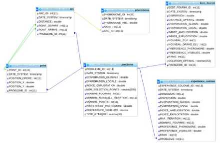
Fig.1. ACS-CKC Database Schema

•   anr: The preference of the pheromone for the graph of dimension n and in the research stage r.

The simulation runs at an estimated time of 10 minutes 20 seconds, on an 8 GB RAM machine, with a 2.00 GHz 4 - core processor and SSD storage Disk for fast access.

The evolution of the parameters a, P , and S as a function of the experiments and the research stages are

represented in the following graphs.

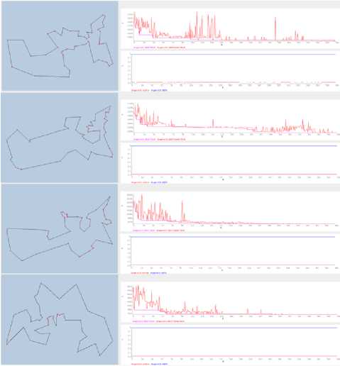
Fig.2. The 1 ^st, 20"^I,40"^I and 70"¹ experience of ACS Normal

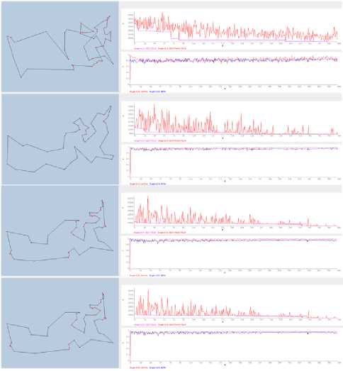
Fig.4. The 1 ^st, 20 ' ^A ,40 ^tAand 70 "' experience of ACS-CKC with dynamic ^ 0

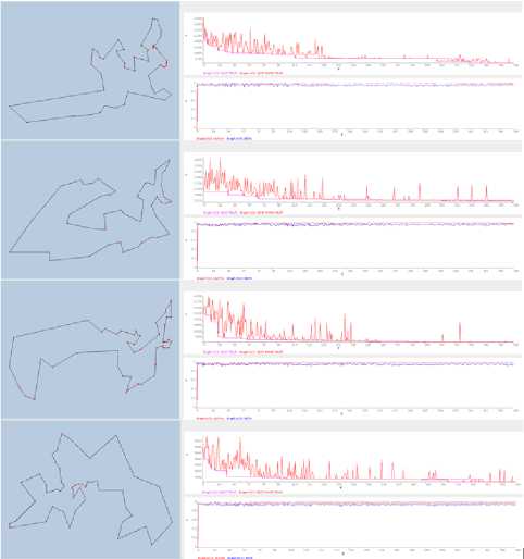
Fig.3. The 1 ^st, 20 ^tA ,40 ^tAand 70 ^Ift experience of ACS-CKC with static ^ 0

elite

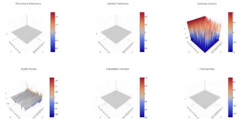
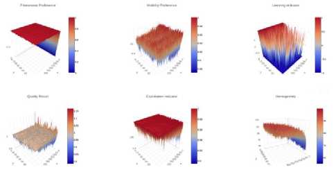
Fig.5. a, p, learning indicator, ^nr , ^ 0 and standard deviation graphs ^p nbest

in terms of n and r for ACS Normal

pelite

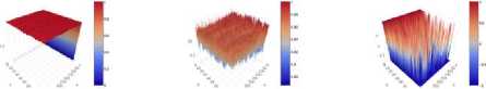
Fig.6. a, P, learning indicator, ^nr , q₀ and standard deviation graphs C nbest

in terms of n and r for ACS-CKC with static q 0

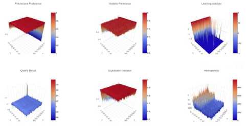
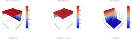
pelite

Fig.7. a, p , learning indicator, ^nr  , q o and standard deviation graphs

^ nbest

capital of the US of the order of magnitude of the distances 10000) will obviously give a discontinuity of the dispersions of the results during the simulation.

So our first quality criterion proposal is not the best one, and it needs to be improved by developing a variant that requires the following:

• •    It depends on many of the nodes of the graph.

• •    It is invariant by a change of scale.

• •    It depends on the metric of the graph.

in terms of n and r for ACS-CKC with dynamic q ₀

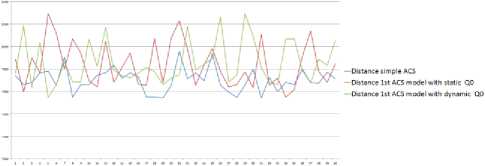
Fig.8. Optimal distances obtained by ACS Normal, ACS-CKC with static q ₀ and ACS-CKC with dynamic q ₀

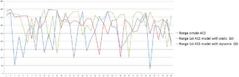
Fig.9. Optimal stages obtained by ACS Normal, ACS-CKC with static q o and ACS-CKC with dynamic q o

A. The Construction of the Homogeneity Level of a Colony

We have seen that the mechanism of optimization by the colony of ants has a tendency to have, in convergence, a common solution between all agents of the colony. During the research, the ants deposit the pheromone on the roads of quality, in order to guide the other members of the colony to follow them, and in the end the colony tends to adopt the same solution which will be considered the better solution.

Suppose the colony ends a research stage. Let an arc (i,j) in the graph Gr , we define X G _r as a function which expresses the frequency of use of the arc (i,j) by the member of the colony, that it will present the number of ants whose the arc (ij) is an element of the solution. So formally:

^Gr —* 10,^1

(i,j) ^ X G _r(i,j) = card({k E [0,K] ,

i E 0 „ _r and j

j choosen }) ^-

• VI. Analysis of the Improved first Model

The analysis of the results of the simulation models shows a close evolution with respect to the optimal distance found between the normal ACS and the proposed models.

Note that the two models of the knowledge center have a tendency to have the same results, but an analysis of the speed of convergence towards the optimal result shows an advantage for the exploitation of all the parameters in average, and also it makes a stable pattern in term of results.

In another analysis, at first glance, it seems that there is a stability of the a,f preference values during the 40 experiments, but the analysis of the 3d perspective of the dispersion values and the quality shows a discontinuity between Phase of the random experiments and the last 40 experiments which concern a single graph.

A simple analysis of proposed data for the simulation shows that there is a lack of modeling of the quality value, which is based on the dispersion of the search results. Indeed, the dispersion has the unit of distance (the meter in our case), and the fact to test first on random samples of the example att532.tsp (which proposes a drilling problem of order of magnitude distances 300) and then to approach the example berlin52.tsp (which proposes the

We define V^r a function that binds each ant to its degree of commitment to follow the policy of the colony. Indeed if an ant adopts the same strategy as that of the other members of the colony, then its degree of commitment will be better, if not, i.e. It diverges in terms of choice of the arcs compared to the other members, it will have a mediocre score. Formally:

• 10, K] — N

k^v^r(k)=      ^       x Gr (i^i).   (26)

^® Пг _and j=j^l _c ^k _h ^r _oosen

Then, finally, we define fnr as the degree of the homogeneity of the colony in terms of the strategy adopted by the members of the colony by:

к

F „ _r = ^ V^r(k) .               (27)

k=1

• B.    Analysis Of, Г_пг For A Homogeneous Strategy And A Dispersed Strategy Of The Colony

We have seen previously in the analysis of the old dispersion parameter that there was an anomaly with respect to the scaling of the graph. Our new modeling is based on a construction based on an abstraction linked to the basic choices of the ants, and not to the associated values. We will then observe the behavior of our variable Гпг in the two most extreme situations, where the total orientation of the members of the colony is directed towards a single solution (a totally homogeneous strategy), and the second situation where each member of the colony adopts a totally different solution to the other members (totally dispersed strategy).

• •    A totally homogeneous strategy : In such a situation, the colony adopts a single solution namely 0 ^ _r

  r.

  
  

  i E 0_nr and.

  
  

  WJ) EAGr'

  
  

  '7    J choosen

  
  

  ( ie^ kr

  {      or

  ^ ^J ^ ^jchoosen

  
  

— X Gr (i,j) = К

I

^XUi,J) = 0

Then, all the members of the colony have an engagement score expressed by:

V к E 10, K]Vr(k) = nK ।(29)

And the degree of homogeneity of the colony is thus expressed:

кк

Г„г = ^Vr(k) =^nK = nK2.(30)

k=1k=1

• •    A totally dispersed strategy: In such a situation, the colony members adopt disjoint solutions, it is assumed that there will be enough arcs for the ants to have such a possibility.

V(i,j) E AGr XGr(i,j) = 1 or XUi,D = 1 I(31)

Then, all the members of the colony have an engagement score expressed by:

V kE[0,K] Wr(k) = n I(32)

And then the degree of homogeneity of the colony is given by:

кк

Г„г = ^ vr(k) =^n = nK i(33)

k=1k=1

In conclusion, between the homogeneous strategy and the dispersed strategy, we always have nK²,nK, so the more homogeneous the strategy, the greater is its value, and we always Г^ E [[nK, nK²].

And we define the new relation of order < for <^ 1 = (H 1 , Г 1 ) and <^₂ = (H₂, Г₂) by the relation:

< 1 < < 2 ^ ^ i > H 2 or (H 1 = H 2 and Г 1 < Г 2 ).  (34)

• C.    Simulation And Results

The simulation of the second ACS-CKC model precedes with the same conditions, such as the problem cartridges, the hardware processing capacity. The results are indicated in the top graphs.

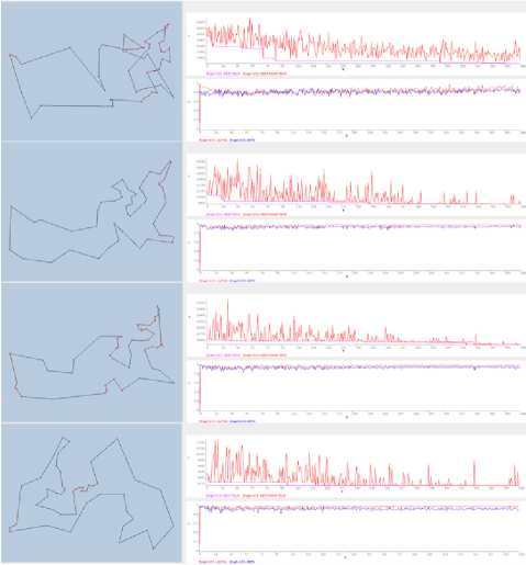
Fig.100. The 1 ^st, 20 ^Ift , 40 ^Iftand 70 ^Ift experience of ACS-CKC 2 ^nti model with static Q o

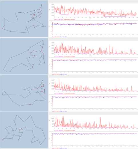
Fig.11. The 1 ^st, 20 ^tft ,40 ^t,land 70^ experience of ACS-CKC 2 ^nd model with dynamic Q 0

pelite

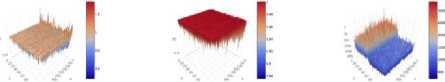
Fig.12. a,p, learning indicator, nr , qo and standard deviation ^nbest graphs in terms of n and r for ACS-CKC 2nd model with static q0

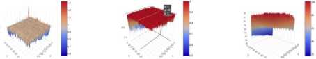
£elite

Fig.13. a,P, learning indicator, nr , qo and standard deviation ^nbest graphs in terms of n and r for ACS-CKC 2nd model with dynamic q0

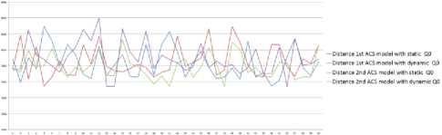
Fig.14. Optimal distances obtained by 1 ^st and 2 ^ndACS-CKC model with static and dynamic q ₀

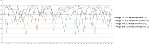
Fig.15. Optimal stages obtained by 1 ^st and 2 ^ndACS-CKC model with static and dynamic q o

The analysis of the results obtained by the second model shows a new evolution on the homogeneity and the learning index variations. We note that the homogeneity evolution presents a smooth continuous variation which will end up being maximized at the end of the learning period. This variation does not depend on the nature of the graph or its metric, something which is not verified in the first model.

Due to the new variation in homogeneity, the colony finds better configurations, which is not the case in the first model that uses metric dispersion to express homogeneity.

• VII.    Statistical Analysis of Models with a Collective Knowledge Center

The comparison of the results between the first model and the second shows a slight advantage of the first model, in terms of the optimal distance found. But, statistically, we can prove that the four models: ACS-CKC 1^st model with static and dynamic q_0 , and ACS-CKC 2^nd model with static and dynamic q_0 , and the classical ACS model have a tendency to give the same results.

Indeed, we performed a static analysis on 33 graphs of TSP, comparing, on the one hand, the four models that illustrate our approach of dynamic parameterization, and the basic model ACS.

Statistical analysis [ANOVA test (for a level of significance α = 0.01), Tukey Tests (confidence level = 99.89%), Dunnett Simultaneous Tests (confidence level = 99.73%), Hsu Simultaneous Tests (confidence level = 99.44%), shows an equivalence between the five models to more than 99%.

Table 1. Statistical Analysis Graphs

a280.tsp	eil76.tsp	lin105.tsp
att48.tsp	kroa100.tsp	lin318.tsp
berlin52.tsp	kroa150.tsp	pr76.tsp
dantzig42.tsp	kroa200.tsp	pr107.tsp
eil101.tsp	krob100.tsp	pr136.tsp
eil51.tsp	krob150.tsp	ch150.tsp
st70.tsp	krob200.tsp	pr124.tsp
pr152.tsp	ts225.tsp	pr144.tsp
pr226.tsp	tsp225.tsp	rat195.tsp
pr264.tsp	bier127.tsp	pr299.tsp
rat99.tsp	ch130.tsp	rd100.tsp

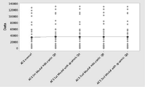
Fig.16. Individual value plot of normal ACS, ACS-CKC 1 ^st and 2 ^nd model with static and dynamic Q o

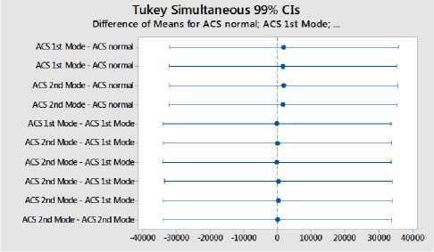
Fig.17. Tukey simultaneous 99% CIs for normal ACS, ACS-CKC 1 ^st and 2 ^nd models with static and dynamic q ₀

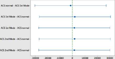
Dun nett Simultaneous 99% Cis

Level Mean - Control Mean for ACS normal; ACS 1st Mode;

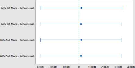
If an interval does not contain zero, the corresponding mean is significantly different from the control mean.

Fig.18. Dunnett Simultaneous 99% CIs for normal ACS, ACS-CKC 1 ^st and 2 ^nd model with static and dynamic q ₀

Hsu Simultaneous 99% Cis

Level Mean - Smallest of Other Level Means for ACS normal; ACS 1st Mode;

If an interval has zero os an endpoint, the corresponding means are significantly different.

Fig.19. Hsu Simultaneous 99% CIs for normal ACS, ACS-CKC 1 ^st and 2 ^nd model with static and dynamic q ₀

• VIII.    Conclusion

In conclusion, the approach with Collective Knowledge Center provides comparable results to those of the classic ACS alternative. However, our approach has many advantages, including the most important ones:

• •    It offers the possibility to carry the optimal configuration like a data briefcase. This briefcase is exportable, that is to say, it can be used in different contexts and dimensions of graphs. In

addition, this briefcase is scalable, that is to say, that every time it is used, it will improve itself, by collecting the new optimal configurations.

• •    It also shows behavior stability, both in terms of the results obtained, or in the solutions research evolution.

• •    It can be seen as an alternative to a machine learning model using reinforcement learning approach, applied to a multi-agent system; Namely, the ant colony system.