A New Classification Algorithm for Data Stream

Published Online July 2011 in MECS

In many fields, such as statistics, artificial intelligence, machine learning, and other disciplines cross discipline, data mining in recent years is becoming a hotspot. Various data mining techniques have been proposed and widely used in order to find useful information from a large number of complex data .With the large number of data produced, the data need to be addressed in one day is to millions or even no limit to the rate of growth. How to mine useful information from these continuous data streams, is becoming the new challenges we had to face [1-9].

At the early stage the data streams originated in the financial markets. Today, the data streams widespread in the Internet, monitoring systems, geology, meteorology, sensor networks and other domain. The data stream is very different with the traditional static data. The data stream is infinite amount of data ， data continuous arrived and can only be read for one or a few times. So the faster method of data stream mining need to be updated.

Data-stream mining is a technique which can find valuable information or knowledge from a great deal of primitive data. Unlike mining static databases, mining data streams poses many new challenges [10].

Data stream has different characteristics of data collection to the traditional database model. Such as the date of data stream continuous generation with time progresses ， and the data stream is dynamic ， and the arrival of the data stream can not be controlled by the order. The data of Data stream can be read and process based on the order of arrival. The order of data can not be changed to improve the results of treatment.

Therefore, the processing of the data stream requires ： First, each data element should be examined at most one time, because it is unrealistic to keep the entire stream in the main memory. Second, each data element in data streams should be processed as fast as possible. Third, the memory usage for mining data streams should be bounded even though new data elements are continuously generated. Finally, the results generated by the online algorithms should be instantly available when user requested.

• A.    Data Stream

Compared with traditional data collection ,the data stream is a real-time, continuous, orderly , time-varying, infinite tuple. A data stream has the following distinctive features: a) orderly, b) cannot reproduce, c) high-speed, d) infinite, e) high dimensional, f) dynamic.

Let us now describe the concept of data stream:

Let I= { i 1 ,i 2 ,…,i m } be a set of literals, called items. An itemset is a subset of I . An itemset consisting of m items is called a m-itemset. Let us assume that the items in an itemset are in lexicographical order. A transaction is a tuple, (tid, itemset) , where tid is the ID of the transaction.

A transaction data stream DS= { B 1 , B 2 , … , B N , … } be an infinite sequence of blocks, where each block is associated with a block identifier n, and N is the identifier of the latest block B_{N .} Each block Bi consists of a set of transactions, that is, Bi=[T 1 , T 2 , …, T k ], where k>0. Hence, the current length of the data stream is defined as CL=|B 1 |+|B 2 |+…|B N | .

The frequency of an itemset, X , denoted as freq(X), is the number of transactions in B that support X. The support of X is defined as fre(X)/N , where N is the total number of transactions received. X is a Frequent Itemset (FI) in B , if sup(X) >= minSupport , where minSupport (0<=minSupport<=1) is a user defined minimum support threshold.

There are many algorithms for mining data stream have been proposed. According to the processing model on the data stream, we can classify the research work into three fields: landmark windows, sliding windows and damped windows. Manku and Motwani[11] proposed a single-pass algorithm, Lossy Counting, to mining frequent itemsets, and the algorithm is based on a well known Apriori-property. Yu et al. [12] proposed an algorithm, FDPM, which is derived from the Chernoff bound, to approximate a set of FIs over a landmark window. Li et al.[13] propose a single-pass algorithm, DSM-FI, to mine all frequent itemsets over the entire history of data streams. Pedro Domingos and Geoff Hulten [14] described and evaluated an algorithm, VFDT, to predict the labels of the records it received.

Classification of data stream mining is a challenging area of research. There are many problems to be solved, such as Handling continuous attributes, Concept drift, Sample taken question, Classification accuracy problem, Data stream management and Pretreatment of the data stream.

1)Handling continuous attributes

When classification of Data Stream face the real-time and memory limit, the reach of how to compute the evaluation function more quickly, how to more effectively compressed storage properties worth further study and how to more effectively compressed storage properties deserves further study.

• 2)    Concept Drifts

Mining concept drifts from data streams is one of the most important fields in data mining. The reach of how more rapidly and accurately judge concept drift, how to effectively use concept drift acquisition, save and heavy use concept, and the trend of concept drift needs to seriously study.

• 3)    Sample sampling

Although there is Hoeffding inequality for sampling methods, how to get better with less precision of the sample, remains a problem worthy to study.

4)Classification accuracy

High classification accuracy is the goal of all classification algorithms. How to improve the classification accuracy is very important research.

5)Data Stream management

Traditional database technology has greatly promoted the development of information technology, but traditional technology look powerless to Data Stream.

• 6)    Pretreatment of the Data Stream

Pretreatment of the Data Stream also need to consider. The reach of how to design a lightweight preprocessing algorithm to guarantee the quality of mining results is very important.The pretreatment of the Data Stream occupies most if the runing time, and how to Decrease running time is also important.

7)Re-use of traditional classification methods

Traditional classification is Decision Rules, Bayesian classification, Back-propagation method, Related classifications, K nearest neighbor classifier, Example based reasoning, Evolutionary algorithm, Rough set method, Fuzzy set the legitimate and so on. The current study was applied some of these methods to data stream. How to use the characteristics of the data stream for the application of these methods will be very valuable.

• B.    Associative Classification

Classification has been studied for many years, it got extensive research of different subjects, including statistics, pattern recognition, machine learning, data mining, etc. It is one of the most essential tasks in data mining and machine learning area. Classification mainly find meaningful information to meet the needs of the user association rules from data. Many effective models and algorithms have been proposed to solve the problem in different aspects, such as support vector machine, decision tree, rule-based classifier, etc.[15].

Different from some traditional rule-based algorithms, associative classification tries to mine the complete set of frequent patterns from the input dataset, given the user-specified minimum support threshold and/or discriminative measurements like minimum confidence threshold. For example, Apriori[16] and FP –growth[17] are now widely used

Association rules proposed by Agrawal etc. The mining of Association rules is a very important research of data mining ， which used to find relationship between Itemsets in the database. Simply ， Association rules is used to describe the extent of interaction between attributes. With the large amount of data continuously collected and stored ， for many people in the industry from their database are increasingly interested in mining association rules. Business transaction records from a large number of interesting relationship was found can help many business decision making. Such as the classification of design, analysis of cross-shopping and the fire sale.

Let I = { i 1 , i 2 , ......, i m } be a collection of items.

Task-related data set D is a collection of database transactions ， Where each transaction T is a collection of items ， and T ⊆ I. Each transaction has an identifier, called TID.

Let A is a Itemset ， and T contain A ， and only if A ⊆ T

Association rule is the implication of the form A B ， where A ∈ I ， B ∈ I ， and A ∩ B = Φ . For the association rule A => B.

Support ( A=>B ) =P ( A ∪ B ) .

Confidence(A=>B) = P(B | A) =support(A ∪ B)/support(A).

Lift(A =>B) = support(A ∪ B)/support( A) × support( B).

Support is percentage of D which contain A or B, is a measure of the importance of association rules ， and explain this rule in all things have much representative. If support larger, association rules are more important. If itemsets meet the minimum support (min_sup), then it called frequent itemsets.

Confidence is percentage of D which contain A or B, is a measure of the accuracy of association rules. When predicting , Conf idence is a natural choice. It reflects that the premise of A given the incidence of B.

Lift sometimes referred to as Interest, it is the rate between probability of A and B happen at the same time and probability of on the assumption that A and B independent premise A and B also happened. Lift used to measure the association between A and B with A and B are independent degree of deviation. If Lift close to 1, A and B are independent. If Lift is less than 1, this rule is not very meaningful. Lift the greater the practical meaning of the rules the better.

In recent years, Classification of association rules applied to obtain good results. These methods mainly excavate to the training set and get some high quality rules, then build classification according to these rules, and forecasting the new example of label.

Let D be the dataset. Let I be the set of all items in D and C be the set of class labels. We say that a data case di ∈D contains X ⊆ I, a subset of items, if X ⊆ di. A class association rule (CAR) is an implication of the form X→c, where X ⊆ I, and c∈C .

A test instance is classified later using classifier trained based on the mined patterns. Bing Liu et al. [18] first proposed the AC approach, named classification based on association algorithm (CBA), for building a classifier based on the set of discovered class association rules. CBA is one of the most classical associative classification algorithms. Empirical results show that associative classification algorithm could provide better classification accuracy than other algorithms on categorical datasets. However, this approach takes a great amount of running time in both pattern mining and feature selection, since most of the mined frequent patterns are not the most discriminative ones and will be dropped later.

The difference between rule discovery in AC and conventional frequent itemsets mining is that the former task may carry out multiple frequent itemsets mining processes for mining rules of different classes simultaneously. Data mining in associative classification (AC) framework usually consists of two steps:

• (1)    Generating all the class association rules (CARs) which has the form of iset ＝> c, where iset is an itemset and c is a class.

• (2)    Building a classifier based on the generated CARs. Generally, a subset of the association rules was selected to form a classifier and AC approaches are based on the confidence measure to select rules [19].

Most of the algorithms shown above were used for finding frequent itemsets. Since the foundation of associative classification is frequent pattern mining, we also introduce the definitions and notations related to frequent pattern mining. Some of them were used to classify the data streams with a decision tree.

We present an approach to mine class association rules and then to make a classifier in this paper. Classifying a data stream with an association classifier is a newly explored area of research, which may be viewed as a further extension to the earlier work on mining frequent itemsets over data stream.

• II.    associative classification on data streams

• A.    Problem Definitions

A data stream is a large number of unconstrained data elements. Due to the unique characteristics of streaming data, most one-pass algorithms have to sacrifice the correctness of their analysis results by allowing some errors. Hence, the True support of an intemset X, denoted by Tsup(X) , is the number of transactions seen so far in which that itemsets occurs as a subset. The estimated support of the itemset X, denoted as Esup(X) , is the estimated support of X stored in the summary data structure constructed by the one-scan approaches, where Esup(X)<=Tsup(X) . An itemset X is called a frequent itemset if Tsup(X)>=Minsupport*CL.

Therefore, given a user-defined minimum support threshold minSupport (0<= minSupport <=1) and a data stream DS, our goal is to develop a single-pass algorithm to classify the streaming data in the landmark windows model using as little main memory as possible.

Input: DS---a data stream in which each record has N items.

S window ---the window size, S window =| Bi |. minSupport--- Support threshold.

Output: M---a classifier with a lot of association rules whose confidence are great than 50% and support value great than minSupport.

Method:

Initial the rule memory M= Φ

Do

Read in a data block Bi={T1, T2, …, Tk} m=0; Am=Φ          //Clear the set of candidate itemsets A

Am+1=Gen(Bi, Am)    // Generate n candidate frequent itemsets,

// Itemset₁, Itemset₂,…, Itemset_n, //each Itemset i in A has 1 items.

While A ≠Φ

For i=1 to n

S=Supp( Itemset i )      //Calculate the support of Itemset i

If S>= minSupport then

M ← M+ Itemset_i   //Put the itemset into memroy

Endif

Endfor m=m+1

A m+1 =Gen(Bi, A m )   //Generate the (m+1) generation A

Endwhile

M=Rank(M)           //Rank rules by their confidence values

M=Decay(M)         //Decay the rules in memory

While

Figure 1. The proposed associative classification algorithm.

• B.    Associative Classification Algorithm for Data

Stream

The figure 1 is our the whole algorithm. The algorithm accepts two user-specified parameters: one is the support threshold minSupport and another is the window size Swindow=| Bi |. Let N denote the current length of the stream, i.e., the number of records seen so far. Every time received a record, our algorithm can forecast its class label based on the association rules extracted from the records before. Each of the rules has a estimated support Esup(X), whose value is great than minSupport.

For a given data block B i , the first pass of the algorithm counts item occurrences to determine the frequent 1-itemsets. As long as the set of 1-itemsets was not empty, the algorithm subsequently carry out the next pass to find frequent (m+1)-itemset. When the algorithm obtains all of the frequent itemsets, it will calculate the confidence of the rules and sort them in the memory. Then, if there is a request of classification, the classifier will predict the class label of a record. At the bound of block B_i, the memory rules will be pruned and the rules with low support value will be deleted.

• C.    Funtions and Data Structure

• 1)    Data struture M

The data structure M is a set of entries of the form (itemset, fclass(1), fclass(2),…, fclass(i), t), where itemset is a subset of conditional attributes, fclass(i) is an interger representing the approximate frequency of class attributes i, and t is the number of the data blocks in which the itemset appeared firstly. Initially, M is empty. Whenever a new association rule (itemset, class(i)) arrives, we examine M to see whether an entry mj already exists or not. If exists, we update the entry by incrementing its corresponding frequency fclass(i) by one. Otherwise, we create a new entry of the form (set, fclass(1), fclass(2),…, fclass(i), t). The parameter t is the number of the data block and fclass(x) is the frequency of class x.

• f class(x ) =0 (class(x) ≠ class(i))

• f class(x )       =1 (class(x) =            class(i))

• 2)    Function Gen(B x , A m )

The Gen(Bx, Am) function takes as argument Am, the set of all frequent m-itemsets. It returns a superset of the set of all (m+1)-itemsets. The function works as follows [20]:

• a)    Step 1, we join A m with A m :

• Insert into A m+1 :

• Select p.item 1 , p.item 2 , …, p.item m , q.item m From A m p, A m q

• b)    Step 2, we delete all itemsets a ∈ A_m+1 such that some m-subset of a is not in A m :

Forall itemsets a∈ A m+1 do

Forall m-subsets s of a do

If NOT (s ∈ A m ) then

Delete a from A m+1;

• 3)    Function Supp(Itemset x )

The function Supp(Itemsetx) was used to calculate the support value of Itemsetx. The value of the function was calculated like this:

Supp(Itemset x )= MAX(f class(1) , f class(2) ,…, f class(i) )/N (2)

Where N is the number of current data block.

• 4)    Function Rank(M)

The function Rank(M) was used to sort the rules in M with their confidence values. The confidence value of a entry in M was calculated like this:

Confidence(mi)=MAX(f class(1) , f class(2) ,…, f class(i) )/ (f class(1) ,

• 5)    Function Decay(M)

The function Decay (M)

+f class(2) ,   +…+,  f class(i)   )

was used to delete some

entries at the boundary of a data block. If the expression below is true, the entry will be deleted from the memory M. N is the number of current data block.

MAX(f class(1) , f class(2) ,…, f class(i) )+minSupport*(t-1) *CL

< minSupport*N*CL    (4)

• III.    EXPERIMENTS

In this section, based on past experience, we provided a formal model of associative classification and further examine how such algorithm can be applied in data stream mining. We have conducted an experiment on a 2.93 GHz Pentium PC with 1GB of memory running with Microsoft Windows XP to measure the performance of the proposed approach. The datasets used in the experiment are obtained from the UCI Maching Learing Repository[21]. In order to compare our algorithm with other classification algorithms and make the evaluation more credible and reliable, we choose some large datasets from UCI. The Entropy method was used in the progress of discretization of continuous attributes[22].

• A.    Effects of Parameters

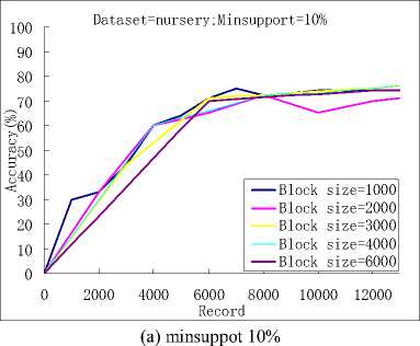
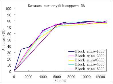
In this paper we investigated the effects of the different block sizes on the effectiveness and efficiency of the algorithm and found that the accuracy of the algorithm was not affected obviously by it. But the number of the rules found and the time cost were affected by it largely.

(b) minsuppot 5%

0    2000   4000   6000   8000 10000 12000

Record

0    2000  4000   6000   8000 10000 12000

Record

(c) minsuppot 10%

(a) Dataset=nursery ; minsuppot 10%

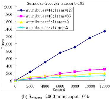
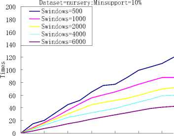
Figure 3. The run time of the classification algorithm.

Dataset=nursery;Minsupport=5%

Block size=1000       Block size=2000

Block size=3000       Block size=4000

Block size=6000

(d) minsuppot 5%

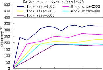
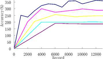
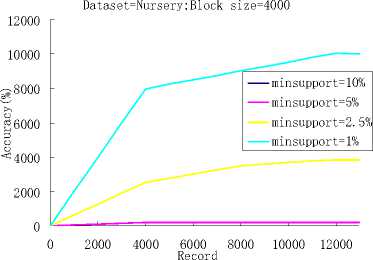
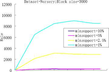
Figure 2. The accuracy of the classification algorithm and the number of the rules found.

Through our previous research,we further investigated the effects of different block sizes on the time cost by the algorithm and found that with the same dataset, as the increasing of the block size, the total run time becomes more and more long. With the different dataset, the run time was decided mainly by the number of attributes and the number of the items of the dataset. We can see this from Fig.3, the numbers of the attributes of the four datasets, Poke and Adult, are 8, 6, 10 and 14. And the numbers of the items of them are 27, 40, 85 and 127. Although, the support thresholds and the block sizes of them are the same, the run time of them are very different and it increased obviously with the increasing of the item and attribute.

The figure 2 is the computational results, we can seen that when the initial data block size was set to 1000, 2000, 3000, 4000 and 6000, and minimum support threshold was set to 10%, and when the initial data block size was set to 1000, 2000, 3000, 4000 and 6000, and minimum support threshold was set to 5% . So we got the similar forecast results. However, the numbers of the found rules are very different. When the block size getting larger, the number of the found rules became smaller.This is because that, although we delete some entries at the boundary of a data block, there still are some un-frequent rules in the memory and they will be deleted in the later decay step. The larger the data block size is, the less the number of un-frequent rules exists.

(a) Dataset=nursery ； Accuracy Size 2000

Dataset=Nursery;Block size=2000

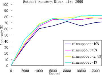
minsupport=10% minsupport=5% minsupport=2.5% minsupport=1%

0    2000  4000   6000   8000 10000 12000

Record

(f) Dataset=nursery; Accuracy Size 4000

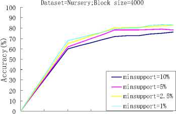
Figure 4. The effects of different support thresholds.

(b) Dataset=nursery; Accuracy Size 2000

0    2000 4000 6000 8000 10000 12000 14000

Record

When the block size was set to 2000, we tested the performance of the algorithm with the different support thresholds, and when the block size was set to 3000 and 4000, we also tested the performance of the algorithm with the different support thresholds. As it can be seen from Fig.4, the block size of figure (a) and (b) was set to 2000, figure (c) and (d) was set to 3000, and figure (e) and (f) was set to 4000,with the decreasing of the support threshold value, the more accurate classification result we can get. But, at the same time, more classification rules will appear in our classifier, it means more run time.

(c) Dataset=nursery; Accuracy Size 3000

0    2000 4000 6000 8000 10000 12000 14000

Record

(d) Dataset=nursery; Accuracy Size 3000

0     2000   4000   6000   8000   10000 12000

Record

(e) Dataset=nursery; Accuracy Size 4000

• B.    Comparision with different algorithms

  Here, we compared the CBA algorithm [8] and AC-DS algorithm. The minimum confidence was both set to 50%., and the data block size was set to 1000. The support thresholds of the two algorithms were shown in the Table.1.

Column 1: It lists the names of the 6 datasets.

Column 2: It lists the number of attributes in the dataset.

Column 3: It lists the number of classes in the dataset

Column 4: It shows the support threshold used in the algorithm.

Column 5: It shows the classification accuracy of the algorithm CBA.

Column 6: It shows the number of the records which had to been read in the memory by CBA.

Column 7: It shows the classification accuracy of the algorithm AC-DS.

Column 8: It shows the number of records in a data block which was read in the memory by AC-DS.

We test the adult, digit, Letter, Mushroom, Nursery, Krkopt, 6 data sets which come from UCI Machine Learning Repository. As can be seen from table.1, the mean accuracy of the two algorithms is very similar, but the memory used by CBA is obviously greater than AC-DS. Since CBA is a classification algorithm for static dataset and AC-DS is a classification algorithm for mining data streams, the more total time cost by AC-DS than CBA should be think acceptable as long as the two accuracy rates of them are similar and the memory cost by AC-DS is in a special limit.

TABLE I. C omparision with different algorithm

Dataset	#attr	#class	#supp	CBA		AC-DS
				#accu	#mem	#accu	#mem
Adult	14	2	10%	83.7%	48842	82.1%	1000
Adult	14	2	5%	83.9%	48842	81.9%	1000
Adult	14	2	1%	85.3%	48842	83.7%	1000
Digit	16	10	10%	78.7%	10992	75.6%	1000
Digit	16	10	5%	86.0%	10992	83.4%	1000
Digit	16	10	1%	87.2%	10992	86.0%	1000
Letter	16	26	10%	59.2%	20000	62.8%	1000
Letter	16	26	5%	69.0%	20000	67.4%	1000
Letter	16	26	1%	70.1%	20000	68.6%	1000
Mushroom	22	2	20%	94.0%	8124	91.4%	1000
Mushroom	22	2	10%	96.4%	8124	93.2%	1000
Mushroom	22	2	2%	96.6%	8124	94.6%	1000
Nursery	8	5	10%	89.9%	12960	90.4%	1000
Nursery	8	5	5%	91.5%	12960	89.5%	1000
Nursery	8	5	1%	96.1%	12960	93.8%	1000
Krkopt,	6	18	10%	89.2%	28056	87.4%	1000
Krkopt,	6	18	5%	94.2%	28056	91.8%	1000
Krkopt,	6	18	1%	97.9%	28056	97.1%	1000

• IV.    discussions and conclusion

With the development of information technology, more and more applications produce or receive a steady stream of data streams. Data streams analysis and mining have become a research hotspot.

As each transaction was not processed, we used to read in the available main memory as many transactions as possible .So, we always select a large data block size to process. When the support threshold is fixed, the more the data block size is, the less combinatorial explosion of itemsets takes place.

This paper introduced a kind of mining association of data stream classification. Our algorithm was designed to deal with dataset in which the all data was generated by a single concept. If the concept function is not a stationary one, in other words, a concept drift takes place in it, our algorithm will not output an accurate result.Empirical studies show its effectiveness in taking advantage of massive numbers of examples. AC-DS’s application to a high-speed stream is under way.