A New Measure of Fuzzy Directed Divergence and Its Application in Image Segmentation

Published Online March 2013 in MECS

The concept of fuzziness introduced by Zadeh [7] revolutionized research and development in the area. De-Luca and Termini [8] defined the measure of fuzzy entropy corresponding to Shannon [1] measure of entropy. Bhandari and Pal [9] defined measures of fuzzy entropy corresponding to Renyi [2] entropy and measure of fuzzy directed divergence corresponding to Kullback Leibler [3] divergence measure. Literature on the development of divergence measures has expanded considerably in recent years. Bhatia and Singh [10]

presented a survey of fuzzy information and divergence measures.

Thresholding, a popular tool for image segmentation, is used here for extracting the objects from a picture. If the objects are clearly distinguishable from the background, the threshold values for segmentation can be chosen at the valley points of the multimodal histogram.

Otsu [11] selected the threshold so as to maximize the class separatability, which was based on within class variance, between class variance and total variance of gray levels. A number of excellent investigations on various thresholding techniques are reported in the literature. Kapur et al. [12], Sahoo et al. [13,14], Sahoo and Wong [15], and Brink and Pendcock [16] used information theoretic measures to threshold an image.

Fuzzy set theory is applied to image thresholding to partition the image into meaningful regions. The application of fuzzy notions in image processing has gained importance because of several reasons like (i) imprecision of the gray levels of an image, (ii) ambiguity in some definitions, such as boundaries between the regions, or region textures etc. Thus it is possible to allow the segments to be several fuzzy subsets of the image. The measures like entropy, index of fuzziness and index of non fuzziness can be used as objective functions which may be optimized for image segmentation. Index of fuzziness represents the average amount of fuzziness in an image by measuring the distance between the fuzzy property of an image and its nearest two-tone version. The index of non-fuzziness indicates the amount of non-fuzziness in an image by taking an absolute difference between the fuzzy property of an image and its complement.

Several researchers used fuzzy based thresholding techniques. Pal and Dasgupta [17] introduced a concept of spectral fuzzy sets for finding the membership value and then segmented the image. Huang and Wang [18] assigned the membership value by taking the reciprocal of the absolute difference of pixel and the mean of the region to which that pixel belongs. Ramar et al. [19] used the neural network for selecting the best threshold using various fuzzy measures viz., linear and quadratic indices of fuzziness, logarithmic and exponential entropy. Cheng and Chen [20] used fuzzy homogeneity vectors and fuzzy co-occurrence matrix for image thresholding.

In this paper a new approach to develop probabilistic divergence measures and thereby measures of fuzzy directed divergence is presented. A new measure of fuzzy directed divergence is introduced and some of its properties studied. A new method based on minimization of fuzzy directed divergence using Gamma distribution to determine the membership function of pixels of an image introduced by Chaira and Ray [21] is applied in context with the newly developed measure of fuzzy directed divergence. The proposed methodology involves the minimization of the divergence between the pixels in an ideally thresholded image and actually thresholded image.

This paper is organized as follows. Section II addresses the preliminaries. Section III presents an approach to develop probabilistic divergence measures . In section IV, a new measure of fuzzy directed divergence is presented. Section V deals the application of new measure of fuzzy directed divergence in image segmentation, and section VI contains concluding remarks.

• II.    Preliminaries
  
  2.1    Information Measure

  The measure of information was defined Claude E. Shannon in his treatise paper [1] in 1948.

n

H(P)=∑pi log pi , P∈Γn i=1                                                    (1)

Where

n

is the set of all complete finite discrete probability distributions. To improve upon the weakness of Shannon’s measure in certain situations Renyi [2] took the first step and proposed a parametric measure of information

1 ⁿ

H _α ( P ) =      log ( ∑ p ^α _i ), α ≠ 1, α > 0

• ^{1    - α       i = 1}                             (2)

• 2.2    Divergence Measure

The relative entropy or directed divergence is a measure of the distance between two probability distributions. In statistics, it arises as the expected logarithm of the likelihood ratio. The relative entropy

D(P,Q) is the measure of inefficiency of assuming that the distribution is Q when the true distribution is P . For example, if we knew the true distribution of the random variable, then we could construct a code with average description length H(P). If, instead, we used the code for a distribution Q, we would need H(P) + D(P,Q) bits on the average to describe the random variable. The relative entropy or Kullback-Leibler distance Kullback and Leibler [3] between two probability distributions is defined as np D(P,Q)=∑pi log i i=1           qi                                (3)

A correct measure of directed divergence must satisfy the following postulates:

• a.    D (P,Q) ≥ 0

• b.    D (P,Q) = 0 iff P = Q

• c.    D (P, Q) is a convex function of both

• 2.3    Fuzzy Sets

P = ( p ₁ , p ₂ ,..., p _n ) _and Q = ( q ₁ , q ₂ ,..., q _n )

If in addition, symmetry and triangle inequality is also satisfied by D(P,Q) then it is called a distance measure . Properties (a)-(c) are essential to define a new measure of directed divergence. A parametric measure of directed divergence can also be characterized in terms of its parameter(s).

Definition [7]. Let a universe of discourse X = {x₁, x 2 , x 3 … x n } then a fuzzy subset of universe X is defined as

A = {(x; µ A (x)) / x ∈ X; µ A (x): X [0; 1]}

Where µ A (x): X → [0; 1] is a membership function defined as follow

	0	if x does not belong to A and there is no ambiguity
µ A (x) =	1	if x belong to A and there is no ambiguity
	0.5	if there is maximum ambiguity whether x belongs to A or not

In fact µ A (x) associates with each x ∈ X a grade of membership of the set A. Some notions related to fuzzy sets [7].

Containment ; A ⊆ B ⇔ µ A (x) ≤ µ B (x) for all x

^∈ X

Equality ; A = B ⇔ µ A (x) = µ B (x) for all x ∈ X

Compliment ; A = Compliment of A ⇔

^{µ A ( x )} = 1- µ A (x) for all x ∈ X

Union ; A ∪ B = Union of A and B ⇔ µ ^{A ∪ B} ( x ) = max.{ µ A (x) , µ B (x)}for all x ∈ X

Intersection ; A ∩ B = Intersection of A and B ⇔ µ ^{A ∩ B} ( x ) = min.{ µ_A(x) , µ_B(x)} for all x ∈ X

Product ; AB = Product of A and B ⇔ µ ^AB ( x ) = µ A (x)µ B (x) for all x ∈ X

Sum ; A ⊕ B = Sum of A and B ⇔ µ ^{A ⊕ B} ( x ) = µ A (x) +µ B (x) - µ A (x) µ B (x) for all x ∈ X

• 2.4    Fuzzy directed divergence

Definition [22] . Let a universal set X and F (X) be the set of all fuzzy subsets .A mapping D : F (X) × F

• (X) → R is called a divergence between fuzzy subsets if and only if the following axioms hold:

• a.    D (A, B)

• b.    D (A, B) =0 if A=B

max.{ D ( A ∪ C , B ∪ C ), D ( A ∩ C , B ∩ C )} ≤

• c.    ^{D ( A , B )}                                          for

any A, B, C ∈ F(X)

Instead of axiom (c) if D (A, B) is convex in A and B even then it is a valid measure of divergence.

Bhandari and Pal [9] defined measure of fuzzy directed divergence corresponding to (3) as follow:

D ( A , B ) = ∑ ⁿ µ A ( x i )log ^{µ A ( xi )} + i = 1               ^µ B ( ^x i )

(1 - µ _A ( x _i ))

(1 - µ _B ( x _i ))

n

∑(1 - µA (xi)) log i=1

(3A)

Definition [23]. Let a universal set X and F (X) be the set of all fuzzy subsets .A mapping D: F (X) × F (X) →R is called a distance measure on F(X) if and only if the following axioms hold:

• 2.5 Aggregation operations

The aggregation operation on fuzzy sets is the operations by which several fuzzy sets are combined to produce a single set. e.g fuzzy union and fuzzy intersection are special cases of aggregation operations.

Defnition [10]. An aggregation operation is defined by the function M : [0,1]   → [0,1] verifying

• 1.    M(0,0,0,...0) = 0 , M(1, 1, 1,…,1) = 1 (Boundary Conditions)

• 2.    M is Monotonic in each argument. (Monotonicity)

The use of monotone functions is justified in many decision making contexts, since it ensures consistency and reliability. The boundary conditions here are specified with the assumption that inputs are provided on the unit interval, however in certain cases, inputs naturally expressed on different intervals can be scaled appropriately. If n=2 then M is called a binary aggregation operation.

Aggregation functions are classed depending on their behavior relative to the inputs. The most commonly used in application are averaging functions, which are usually interpreted as being representative of a given set of inputs or input vector.

• III.    An Approach to Develop Probabilistic
  
  Divergence Measure

Let U ( a , b ) and V ( a , b ) be two binary aggregation operators then

D(P,Q)=∑U(pi,qi)-V(pi,qi) I i                                               (4)

Where ^{P , Q ∈ Γ n} as in section II.

is divergence measure.

A* :[0,1]2 → [0,1]

We have        ,         , such that

_*        a + b

A ^*( a , b ) =

and H*:[0,1]2→[0,1]such that

• a.    D (A, B) =D (B, A)

• b.    D (A, B) =0 if A=B

D ( T , T ) = Max A , B ∈ F ( X ) D ( A , B )   ∀ T ∈ P ( X )

c.

• d.    ^{∀ A , B , C ∈ F ( X )} if ^{A ⊂ B ⊂ C} , then

D ( A , B ) ≤ D ( A , C ) _and D ( B , C ) ≤ D ( A , C )

H ^*( a , b ) =

a ² + b ² a + b

are aggregation operations.

Now using these aggregation operators following divergence measure is defined by Bhatia and Singh [24].

n

Dr A P • Q ) = X i = 1

• p ■ q i    P i + q i

. Pi + q_t       ^

у ⁽ Pi - qt ⁾² i = 1 ²⁽ P i + q i )

^ M a u c ^{( x} ) = max .^{ M a ^{( x} ), M C ^{( x )}} = M C ^{( x} )

B ^u c = Union of B and C

^ M b u c ^{( x} ) = ^max .^{ M b ^{( x} ), M C ^{( x )}} = M C ^{( x} )

Taneja [25] has defined several probabilistic divergence measures using this approach. Researchers have defined measures of fuzzy directed divergence corresponding to classical probabilistic divergence measures, a brief review is presented by Bhatia and Singh [24]. In section IV a new measure of fuzzy directed divergence corresponding to (7) is defined.

^A ^ C Intersection of A and C

^ M a n C ^{( x} ) = ^min -^{ M a ^{( x} ), M C ^{( x )}} = M a ^{( x} )

^{B П} C Intersection of B and C

The measure of fuzzy directed divergence between two fuzzy sets corresponding to (7) is defined as follows:

M . ■. ( A , B ) =

^ M b n C ^{( x} ) = ^min - ^{ M b ^{( x} ) M C ^{( x )}} = M b ^{( x} )

Therefore from Eq.(8), we have

MFH. .(A иC,BиC) = 0

HA and

MF. .(A n C,B n C) = MF,,. (A,B)

HA               HA

n

X i=1

⁽ M a ⁽ x. ) - M b ⁽ x АУ

M a ⁽ x ) + M b ⁽ x )   ² - M a ⁽ x ) - M b ⁽ x )

MHF*A*(A, B)

s a valid measure

of

fuzzy directed divergence.

Proof. In order to prove that

^M H ^F * A *

(A,B)

s a valid

measure of divergence three axioms (a), (b) and (c) of fuzzy directed divergence must be satisfied.

MF* *(A,B)

a. From definition of ^{H A}        it is obvious that

W

Hence in set, 1

max.{ M F ,_z ( A и C , B и C ), M F >_z ( A n C , B n C )} <

M _H ^F * _A * ( A , B )

By similar calculations it can be observed that above

WWWW   W inequality also holds on sets 2 ,   3 ,   4 ,   5 and 6 .

MF* *(A,B)

Thus H A        is a valid measure of fuzzy directed divergence.

M _H ^F * _A * ( A , B )   M _H ^F * _A * ( B , A )

and

M^F H . _A . ( A , A) = 0

• b. To prove axiom (c) we divide the X, the universe of discourse into six subsets as follow:

W i = ^{ x | x g X , M a ^{( x} ) <  M b ^{( x} ) <  M C ^{( x )}}

W2 = {x | x g X, Ma (x) < Me (x) < Mb (x)}

W з = ^{ x | x ^g X , M b ^{( x} ) <  M a ^{( x} ) <  M e ^{( x )}}

W4 = {x | x g X, mb (x) < MC (x) < MC (x)}W5 = {x | x g X, Me (x) < Ma (x) < Ms (x)}

W6 = {x | x g X, Me (x) < Mb (x) < Ma (x)}

W

In 1 ,

^{A u} C = Union of A and C

Theorem 2. Following properties can be verified for

MHF*A* (A,B)MF. , (A и B, A n B) = MF.,. (A, B)

• 1 .    HA                  HA

• ₂    M^F H . A .( A , A ) = n ^M A ⁽ x ) = 0 or 1.

  when A is a crisp set i.e when

  
  

_ M^F _H ._z( A , B ) = M^F _H ._z( A , B ) V A , B e F ( X )

HA        HA

Proof. we divide the X, the universe of discourse into two subsets as follows:

Wi = {x | x g X, Ma (x) < Mb (x)}W2 = {x | x E X, Ma (x) > Mb (x)}

The proof can be obtained by performing similar

WW calculations as in theorem 1 on sets 1 and 2 .

M

F(X).

F _{*  *}

^{H A} is not a

distance measure on

Proof. From obvious that

definition of

MF* *(A,B)

^{H A}           it is

and

M H^F * A

, * ( A , B ) M ^F * *

( B , A )

be light intensity, depth, intensity of radio wave or temperature. A digital image, on the other hand, is a two-dimensional discrete function f(x,y) which has been digitized both in spatial coordinates and magnitude of feature value. We shall view a digital image as a twodimensional matrix whose row and column indices identify a point, called a pixel, in the image and the corresponding matrix element value identifies the feature intensity level. Here a digital image will be represented as

M _H ^F * _A * ( A , A ) = 0

F

M × N

= [ f ( x , y ) ] _{M × N}

Next we show that,

M _H ^F * _A * ( T , T ) = MaxA , B ∈ F ( X ) M _H ^F * _A * ( A , B )   ∀ T ∈ P ( X )

Differentiating Eq.(8) partially with respect to ^µ A ^{( x ) and µ} B ^{( x )} respectively we have

∂MF

H*A* = 2µ2 ∂µ      B

-

µ _A - 3 µ _B

+ µAµB

Where M × N is the size of the image and f (x. y) ∈ G_L ={0, 1,..., L-1}, the set of discrete levels of the feature value. Since the majority of the techniques we are going to discuss in this paper are developed primarily for ordinary intensity images, in our subsequent discussion, we shall usually refer to f(x, y) as gray value (although it could be depth or temperature or intensity of radio wave).

∂MF

H*A* = 2µA2 ∂µB

-

µ _B - 3 µ _A

+ µAµB

For points of maxima and minima,

∂MF

_H * _A * _{= 0}

∂ µ _A

and

∂MF

_H * _A * _{= 0}

∂ µ _B

We observe that

H*A* is minimum when µA (x) = µB (x)

and maximum when µB(x)=1-µA(x)=µA(x)

Therefore

M _H ^F * _A * ( T , T ) = MaxA , B ∈ F ( X ) M _H ^F * _A * ( A , B )   ∀ T ∈ P ( X )

Finally we observe that ∀ A , B , C ∈ F ( X )   if

A ⊂ B ⊂ C , then

M_H^F * _A * ( A , B ) ≤ M_H^F * _A * ( A , C ) _and

^M H ^F * A

*

(B,C) ≤ M F* *(A, C)

is not satisfied.

• V. Application of new measure of fuzzy directed divergence in image segmentation

• 5.1    Mathematical modeling of image

An image can be described by a two-dimensional function f(x,y), where (x, y) denotes the spatial coordinate and f(x,y) the feature value at (x, y). Depending on the type of image, the feature value could

Thresholding is one of the old, simple and popular techniques for image segmentation. Thresholding can be done based on global information (e.g. gray level histogram of the entire image) or it can be done using local information (e.g. co-occurrence matrix) of the image. Taxt et al.[26] refer to the local and global information based techniques respectively as contextual and non contextual methods. Under each of these schemes (contextual/non-contextual) if only one threshold is used for the entire image then it is called global thresholding. On the other hand, when the image is partitioned into several sub regions and a threshold is determined for each of the sub regions, it is referred to as local thresholding. Thresholding techniques can also be classified as bi-level thresholding and multithresholding. In bi-level thresholding the image is partitioned into two regions—object (black) and background (white). When the image is composed of several objects with different surface characteristics (for a light intensity image, objects with different coefficient of reflection, for a range image there can be objects with different depths and so on) one needs several thresholds for segmentation. This is known as multithresholding. In such a situation we try to get a set of thresholds (t₁, t₂, ,...,, t_k) such that all pixels with ,i = 0, 1, ..., k: constitute the ith region type (t 0 and t k+1 , are taken as 0 and L-1, respectively). Note that thresholding can also be viewed as a classification problem. For example, bi-level segmentation is equivalent to classifying the pixels into two classes: object and background.

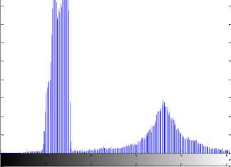
If the image is composed of regions with different gray level ranges, i.e. the regions are distinct, the histogram of the image usually shows different peaks, each corresponding to one region and adjacent peaks

are likely to be separated by a valley. For example, if the image has a distinct object on a background, the gray level histogram is likely to be bimodal with a deep valley. In this case, the bottom of the valley (T) is taken as the threshold for object background separation. Therefore, when the histogram has a (or a set of) deep valley(s), selection of threshold(s) becomes easy because it becomes a problem of detecting valleys. However, normally the situation is not like this and threshold selection is not a trivial job. There are various methods available for this. Here we describe thresholding by fuzzy divergence.

f ( x ) =

Let X  { ^fj , ^{m (} f ij ^{)}   V f} j e X , be an image of

size ^{M x} M having L levels and

f ij be grey level of

(x

—

в

в

(x

v )

Г ( / )

x >  v ; у, в >  0

(I, j)th ■   . ■ v т + M( f„)

,        pixel in X. Let      ^ij

denote the membership

. f  (i, j)th   ■  , ■ Y .     0 < A( fij) < 1

value of ,      pixel in X, where          ij with m( fj )=1 denoting full membership and m(fj )=0 denoting non-membership.

Where ^Y is shape parameter, ^v is location parameter, ^в is the scale parameter and ^Г is the Gamma function given by

X

F(y) = juY—1 e— udu 0

We have the following cases:

Case 1: When v = 0 and в =1, the distribution assumes the form xY—1 exp(—x)

f(x) = —x > 0; Y > 0

^{r ( Y} )                              (12)

which is known as the standard Gamma distribution.

Case 2: When ^v ^ ⁰, ^в =1 and ^Y =1, the Gamma distribution takes the form

For a given threshold value, the membership function derived from the gamma distribution is proportional to the exponential function of negative of the absolute difference between the mean of the region to which the pixel belongs and the pixel gray level. It is thus obvious that this is inversely proportional to the membership value. Let count(f) denote the number of occurrences of the gray level f in the image. Given a certain threshold value t, which separates the object and the background, the average gray level of the background region is given by the relation:

f ^{( x} ) = exp ^{( — ( x — v} ))

Replacing ^v in equation (13) by ^{M o} and ^{M 1} separately from equations (9) and (10), the membership function for the background and object becomes

M o =

t

2 f. count ( f )

f = 0

t

2 count ( f )

f = 0

^{m ( f} j ) = ^{exp( —} c .| ^f j ^— A o^ ff j <  t , for background = ^{exp( —} c .| ^f j ^{— m 1) iff} j > t , for object

and the average gray level of object region is given by

where t is any chosen threshold as stated above. It may be pointed out that in the membership function, the constant ‘c’ is taken to ensure membership of the gray level feasible in the range [0,1] . Here ‘c’ is chosen as

M i =

L - 1

2 f . count ( f )

f = t + 1

L —

2 count ( f )

f = t + 1

c =

(f max

The membership function of each pixel in the image depends on its affinity to the region to which it belongs. The membership values of the pixels are determined using Gamma distribution as described in next section.

The general formula for the probability density function of Gamma distribution is

1

^“

f)

min

where fmin and fmax   are the

minimum and maximum gray level in the image respectively. The absolute value of the distance between the mean of the region to which a pixel belongs and the gray level of that pixel is considered.

For tri-level thresholding, where there are three regions in the image, two thresholds values t 1 and t 2 are selected such that ⁰ <  t ¹ <  t ² <  ^L 1 , where L is the maximum gray level of the image. Extending the concept of bi-level thresholding, the membership function in case of tri-level thresholding will take the form

M ⁽f a ) = ^ex P ^{( -} c i . | f a ^- M o I) f f j <  t i

= exp ^{( -} c i . ^f _y - M i I) f t i <  f j <  t 2

= exp ^{( -} c i. | f j - M i I) zf f j >  t 2

where, ^{M o} , ^{M i} and ^M 2 are the average gray levels for the three regions separated by the thresholds t₁ and t₂ and the constant ‘ c₁’ is like ‘c’ in Eq. (14).

Let ^M A ⁽ f j ) and ^M B ^{( f} ) be the membership

values of the pixels in the image and

f j is ( , j)th

pixel in image A. Then in view of equation (8) fuzzy divergence between A and B is given by

respective regions. From the divergence value of each pixel between the ideally segmented image and the above chosen thresholded image, the fuzzy divergence is found out. It is expected that the membership values of each pixel in the thresholded image should lie close to that of the ideally thresholded image for good thresholding. If a pixel lies in the object/background region, it should contribute more to the corresponding object/background region to which it belongs. In this way, for each threshold, divergence of each pixel is determined according to Eq. (17) and the cumulative divergence is computed for the whole image. The minimum divergence is selected and the corresponding gray level is chosen as the optimum threshold. Here the minimum divergence yields a measure of the maximum belongingness of each object pixel to the object region and that of each background pixel to the background region. After thresholding, the thresholded image leads almost towards the ideally thresholded image.

M * ( A , B ) =

M - i M - i z z z = 0   j = o

( M a ( f ) - M b ( f ))²

+

M a ⁽ f ) ⁺ M b ⁽ X )   ^{2 -} M a ⁽ f ) ^- M b ⁽ f ) J (i6)

For bi-level or multilevel thresholding a searching methodology based on image histogram is employed here. The region between the two successive peaks is the region for searching. If there are more valleys (in case of multimodal histogram) succeeding and preceding peaks of each valley are noted and accordingly the search regions are selected. For unimodal histogram, linear search is employed for selecting the threshold. For each threshold, the membership values of all the pixels in the image are found out using the above procedure. For each threshold value, the membership values of the thresholded image are compared with an ideally thresholded image. Thus equation (16) reduces to

The thresholding algorithm described above is tested on unimodal, bimodal and multimodal images. In order to evaluate the effectiveness of the proposed method, severel images were tested. Here we present experimental result of a bimodal image in png format. Let input image 'Coins' of size i28 ^x i28 (bimodal)'

M * (A, B) =

M - ⁱ M - ^{i (} M a ⁽ f j ) ^- 1 ⁾² Г      i      ₊         i

to z      2      [ Ma (fj) + i 2 - Ma (fj) - i

Fig. 1 and Fig. 2 show a 'coins' image of size i28 ^x i28 and its bimodal histogram. Fig. 3 shows the thresholded image, which is thresholded at gray level 96.

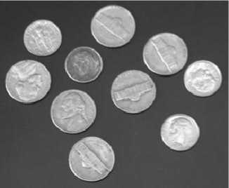
Fig. 1

M - ' M - ^{i (} M a ⁽ f j ) ^{- i)2} Г      i      ₊       i

to z      2      [ Ma (fj) + i i - Ma (fj)_

M - i

=z i=0

M - i

t j=0

i - Ma (fj) . i + Ma (fj),

As the membership values of each pixel in an identically threshold image (which is image B in this case) are taken as unity.

An ideally thresholded image is that image which is precisely segmented so that the pixels, which are in the object or the background region, belong totally to the

0        50        100       150       200       250

Fig. 2

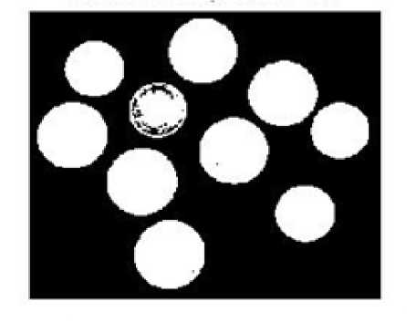
Fig. 3

• VI. Conclusion

In this communication an approach to develop measures of fuzzy directed divergence using aggregation operators is proposed. The proposed measure is not a distance measure but there is possibility of development of distance measures. To add flexibility in applications the divergence (distance) measures may be generalized by using a parameter. In the literature related to image segmentation, the optimum threshold is obtained either by maximizing the fuzzy entropy or by minimizing the fuzzy divergence. Here the optimum threshold is obtained by minimizing the proposed fuzzy divergence. The comparison of proposed measure with the existing measures of fuzzy directed divergence in context of image segmentation is not done, but this is a measure to its own right and can be used for thresholding in some situations because different measures have their suitability in different situations.

The authors would like to thank the anonymous reviewers for their careful reading of this paper and for their helpful comments

• [1]    Shannon, C.E., The Mathematical Theory of Communications. Bell Syst. Tech. Journal, 1948, 27: 423–467.

• [2]    Renyi, A.,On Measures of Entropy and Information. Proc. 4th Berkeley Symp. Math. Stat Probab.1, 1961 :547–561.

• [3]    Kullback,S., R.A. Leibler, On Information and Sufficiency. Ann. Math. Statist., 1951,22 : 79-86.

• [4]    Taneja,I.J.,Generalized Information Measures and their Applications - On-line book :http: //www. mtm.ufsc.br/∼ taneja/book/book.html, 2001.

• [5]    Basseville, M., Divergence measures for statistical data processing.Publications Internes de l'IRISA ,Novembre 2010.

• [6]    Esteban ,María Dolores, Domingo Morales,,A summary on entropy statistic,s”Kybernetika,1995, 31(4): 337–346.

• [7]    Zadeh,L.A., Fuzzy Sets, Information and control, 1965, 8 : 338 - 353.

• [8]    De Luca,A., Termini,S., A definition of non-probabilistic entropy in the setting of fuzzy set theory, Inform. and Control, 1971, 20: 301 - 312.

• [9]    Bhandari, D., Pal,N. R., Some new information measures for fuzzy sets, Information Sciences, 1993, 67: 204 – 228

• [10]    Bhatia,P.K., Singh,S., On some divergence measures between fuzzy sets and aggregation operations (Communicated).

• [11]    Otsu, K., A threshold selection method from gray level histograms. IEEE Trans. Systems Man Cyber.,1979, 9: 62-66.

• [12]    Kapur, J.N., Sahoo, P.K., Wong, A.K.C., A new method of gray level picture thresholding using the entropy of the histogram. Comput. Vision Graphics Image Process, 1985, 29: 273-285.

• [13]    Sahoo, P.K., Soltani, S., Wong, A.K.C., Chen, Y.C., A survey of thresholding techniques. Comput. Vision Graphics Image Process.,1988: 233-260.

• [14]    Sahoo, P.K., Wilkins, C., Yager, Threshold selection using Renyi’s entropy. Pattern Recognition, 1997, 30: 71-84.

• [15]    Sahoo, P.K, Wong, A.K.C., A gray level threshold selection method based on maximum entropy principle. IEEE Ttans. Man Systems and Cyber., 1989, 19 : 866-871.

• [16]    Brink, A.D., Pendcock, N.E.,Minimum crossentropy threshold selection. Pattern Recognition, 1996, 29: 179-188.

• [17]    Pal, S.K., Dasgupta, A., Spectral fuzzy sets and soft thresholding. Inform. Sci,1992,. 65 : 65-97.

• [18]    Huang, L.K., Wang, M.J., Image thresholding by minimizing the measure of fuzziness. Pattern Recognition, 1995, 28 (1) : 41-51.

• [19]    Ramar, K. et al., Quantitative fuzzy measures for threshold selection. Pattern Recognition Lett..2000, 21 : 1-7.

• [20]    Cheng, H.D., Chen, H.H., Image segmentation using fuzzy homogeneity criterion. Inform. Sci., 1997, 98: 237-262.

• [21]    Chaira, T., Ray, A.K., Segmentation using fuzzy divergence Pattern Recognition Letters , 2003, 24: 1837-1844.

• [22]    Couso, I., Janis,V.,Montes,S., Fuzzy Divergence Measures, Acta Univ. M. Belii Math., 2004, 8: 21 – 26.

• [23]    Qing, M., Li, T., Some Properties and New Formulae of Fuzzy Entropy, Proceedings of the 2004 IEEE International Conference on Networking, Sensing & Control, Taipei, Taiwan, March 21-23, 2004: 401-406.

• [24]    Bhatia,P.K.,Singh,S.,Kumar,V., Some New Divergence Measures and Their Properties, Int. J. of Mathematical Sciences and Applications, 2011, 1(3): 1349 - 1356.

• [25]    Taneja,I.J., On Mean divergence measures. available at arXiv:math/0501297v1[math.ST] 19 Jan 2005.

• [26]    Taxt,T.,Flynn,P. J. and Jain,A. K., Segmentation of document images, IEEE Trans. Pattern Analysis Mach. Intell.,1989, 11 (12): 1322-1329

  Authors’ Profiles

  
  
  

Surender Singh, Assistant Professor at School of Mathematics, Shri Mata Vaishno Devi University, Katra (J & K), India. He has taught undergraduate and post graduate students for over ten years. He is also working towards his Ph.D under supervision of Prof. P.K

Bhatia. His research directions include Information, divergence measures and their applications.