A new similarity measure based on simple matching coefficient for improving the accuracy of collaborative recommendations

Published Online June 2019 in MECS

Nowadays, the world wide web (or simply web) serves as an important means for e-commerce businesses. The rapid growth of e-commerce businesses presents a potentially overwhelming number of alternatives to their users, this frequently results in the information overload problem. Recommender Systems (RSs) are the critical tools for avoiding information overload problem and provide useful suggestions that may be relevant to the users [1]. RSs help individuals by providing personalized recommendations by exploiting different sources of information related to users, items, and their interactions [2]. A recommender system facilitates to achieve a diverse set of goals for both the service provider and its end users. The primary goal of an RS on behalf of the service provider is increasing the revenue (by increasing the product sales) while on behalf of the end users, the primary goal of an RS is finding some useful products.

In its simplest form, the recommendation problem can be defined as providing a list of items or finding the best item for a user [3]. Primarily, there are following three broad ways to classify the RSs [4].

• •    Content-based Recommender Systems (CRS): The basic principle of a content-based recommender system is to recommend those items that are similar to the ones liked by a user in the past[5, 6]. For example, if a user listens to pop music, then the system may recommend the songs of the pop genre.

• •    Collaborative Filtering-based Recommender Systems (CFRS): The basic principle of a collaborative filtering-based recommender system is to recommend those items that other similar users liked in the past [7, 8].

• •    Hybrid recommendations:   These methods

hybridize collaborative and content-based approaches for more effective recommendations in diverse applications [9, 10].

Collaborative filtering is the most popular and widely used technique in recommender systems. A detailed discussion on CFRSs is provided in various survey articles published in the past [11, 12, 13]. Article [14] suggests that collaborative recommender systems can be further categorized into two broad classes: memory-based and model-based approaches. Memory-based algorithms [15, 16] are basically heuristic in nature and provide recommendations using the entire collection of rating data available in the UI-matrix. Model-based algorithms [17, 18, 19, 20, 21] learn a model from the rating data before providing any recommendations to users [22].

Among all CFRSs, the neighborhood-based algorithms (e.g., k-Nearest Neighbors) are the traditional ways of providing recommendations [23]. Finding similar users or items is the core component of the neighborhood-based collaborative recommendations since the fundamental assumption behind these approaches is that similar users demonstrate similar interests whereas similar items draw similar rating patterns [24]. Therefore, there exist numerous ways to define the similarity between users or items in the RS literature. Basically, there are two types of neighborhood-based approaches.

• •    User-based collaborative Filtering (UBCF): the main idea is as follows: firstly, identify the similar users (also called peer-users or nearest neighbors) who displayed similar preferences to those of an active user in the past. Then, the ratings provided by these similar users are used to provide recommendations.

• •    Item-based collaborative Filtering (IBCF): In this case, for estimating the preference value for an item i by an active u, firstly, determine a set of items which are similar to item i, then, the ratings received by these similar items from the user u are utilized for recommendations.

One substantial difference between UBCF and IBCF algorithms is that in the former case ratings of peer users are utilized whereas in the latter case active user’s own ratings are used for prediction purpose. With respect to the UI-matrix, UBCF approaches define the similarities among rows (or users) whereas IBCF approaches define similarities among columns (or items) as shown in Fig. 1.

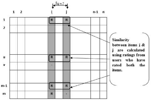
Fig.1. An example scenario for calculating item-item similarity in IBCF.

Traditionally, various statistical measures have been utilized to define the similarity between users and items such as Pearson Correlation Coefficient (PCC)[25, 26], Constrained Pearson Correlation Coefficient(CPCC)[8], Mean Squared Difference(MSD)[8]. Measures from the linear algebra are also utilized to model the similarity, for example, the cosine similarity (COS)[14] calculates the angle between two rating vectors for representing the similarity. Additionally, heuristic-based similarity measures, Proximity-Impact-Popularity (PIP-measure) [27], and Proximity-Significance-Singularity (PSS-measure) [28] are also introduced by the researchers. Authors Bobadilla et al. have proposed various similarity measures by exploiting the different contextual information [29, 30, 31, 32].Patra et al. [33] have adopted the Bhattacharyya coefficient to define a new similarity measure that also manages the data-sparsity problem. Recently, the Jaccard similarity index [34] has been modified to relevant Jaccard similarity [35] for efficient recommendations.

Different types of similarity measures either assist in improving the various RS goals such as accuracy, diversity, novelty, serendipity, etc. or deal with various RS problems such as data sparsity cold start, etc. [36]. However, accomplishing single goal alone is not enough for effective and satisfying users’ experience, therefore, an RS designer has to attain various and possibly conflicting goals. As an example, there are state-of-art model-based approaches which provide better predictive accuracy than the neighborhood-based approaches, however, accuracy alone is not sufficient for effective and satisfying users ‘experience.

Furthermore, the neighborhood-based approaches provide serendipitous recommendations i.e. recommending items that are absolutely different with a factor of lucky discovery. The concept of serendipity augments the notion of novelty by including a factor of surprise [37]. Therefore, finding new similarity measures for neighborhood-based methods is an active thread of research among the researchers. Additionally, the existing CFRS can be easily refurbished by only replacing the similarity measurement module along with the following advantages [2].

• •    Simplicity: very simple to implement and require just one parameter i.e. the number of neighbors, generally.

• •    Efficiency: very efficient in term of performance and memory as there is no costly training phase.

• •    Justifiability:   capable to provide concise

explanations for the recommendations so that users can better understand the system.

Since accuracy is the most discussed and the most examined goal for designing an RS because if a system predicts users’ interests accurately then it would be more useful for the users.

Table 2. The traditional similarity measures

Ref.	Measure Name	Definitive Formula	Methodology (in brief)
[25], [26]	Pearson Correlation Coefficient (PCC)	∑ ( rui - ru )( rvi - rv ) PCC ( u , v ) =     i ∈ Iuv ∑ ( rui - ru )2 ∑ ( rvi - rv )2 i ∈ Iuv                  i ∈ Iuv	It measures the linear relationship between the rating vectors and displays the degree to which two rating vectors are linearly related.
[8]	Constrained Pearson Correlation Coefficient (CPCC)	∑ ( rui - rmed )( rvi - rmed ) CPCC ( u , v ) =     i ∈ Iuv ∑ ( rui - rmed )2 ∑ ( rvi - rmed )2 i ∈ Iuv                     i ∈ Iuv	It adapts the traditional PCC by using the median value (of the rating scale) in place of average rating.
[8]	Mean Squared Difference (MSD)	∑ ( rui - rvi )2 MSD ( u , v ) = 1 - i ∈ Iuv | I uv |	It is the arithmetic mean of the squares of differences between corresponding values of two rating vectors.
[14]	Cosine Similarity (COS)	∑ ( rui )( rvi ) COS ( u , v ) =     i ∈ Iuv ∑ ( r ui )2 ∑ ( r vi )2 i ∈ Iuv          i ∈ Iuv	It measures the cosine of the angle between the rating vectors.
[40]	Adjusted Cosine Similarity (ACOS)	∑ ( rui - ru )( ruj - ru ) ACOS ( i , j ) =      u ∈ Uij ∑ ( rui - ru )2 ∑ ( ruj - ru )2 u ∈ U ij                u ∈ U ij	It modifies the traditional PCC measure for computing similarities between items.

Table 3. The similarity measures based on different contextual information

Ref.	Metric Name	Methodology in Brief	Evaluation Goal	Drawback(s)
[29]	JMSD	The metric is designed by combining two factors: •   mean squared difference (MSD). •    Jaccard index(J)	High level of accuracy, precision, and recall.	Poor Coverage
[32]	SING-metric (Singularity Based)	For each commonly rated item, singularity concerned with the relevant and non-relevant vote is calculated using all the users in the database. Then, a traditional similarity (such as MSD) measure is modulated by the value of the singularity over three subsets of the commonly rated items. Here, the authors utilize MSD as a traditional numerical similarity measure.	Improving the coverage.	Poor Performance due to calculation/updatin g of the singularity values.
[30]	CJMSD	It augments the JMSD measure by adding a term corresponding to the coverage that a user u can provide to another user v.	Combine the positive aspects of JMSD and SING.	Asymmetric measure
[31]	S-measures (Significance Based)	Firstly, three different types of significances (for items, users and useritem pair) are defined Secondly, s-measures between users u and v are defined over the items for which a significance measure can be defined for users u and v. Finally, traditional similarity measures PCC, COS, and MSD are used to define s-measures PCC s , COS s , and MSD s respectively.	Extends the recommendation quality measures along with new similarity measure.	Poor Performance due to calculation/updatin g of the significance values.

Table 1. The notations used

Symbol	Meaning
U	All the users of the system
I	All the items available in the system
R	All the ratings made by the users for the items
S	All possible preferences that can be expressed by the users such as S= {1,2,3,4,5}
r ui	The rating value given by a user u ϵ U to a particular item i
I u	The set of items rated by a particular user u
U i	The set of users who have rated a particular item i
I uv	The set of items rated by both the users u and v i.e. (I u ∩ I v )
U ij	The set of users who have rated both the items i and j i.e. (U i ∩ U j )

Table 4. The heuristic-based similarity measures, PIP, NHSM, and PSD

Ref.	Metric Name	Methodology in Brief	Evaluation Goal	Major Drawback(s)
[27]	PIP	It considers the three factors of similarity, Proximity, Impact, and Popularity for defining the overall similarity between two users u and v.	New user cold-start problem.	PIP score penalizes repeatedly.
[28]	NHSM	It considers three factors of similarity, Pr oximity, Significance, and Singularity and adopts a non-linear function for their computations.	Utilizing local and global rating patterns.	The definitive formula is very complex
[43]	PSD	This measure also considers the three factors of similarity, Proximity (Px), Significance (Sf), and Distinction (Dt) and uses the linear combination method for defining the final similarity measure.	optimal weight combination using PSO algorithm.	High-performance time.

This article proposes a new similarity measure for defining the similarities between users or items in neighborhood-based collaborative recommender systems. Firstly, we have described a way for applying the simple matching coefficient (SMC)[38] and explained how it can be applied to the common ratings between users or items. Secondly, the structural information between rating vectors is modeled using the Jaccard index [34]. Finally, the adapted version of the SMC is combined with the structural information in order to define the similarity between users or items.

We have conducted several experiments to validate the effectiveness of the proposed method against several baseline approaches using benchmark datasets, MovieLens-1M, MovieLens-10M, and MovieLens-20M. Empirical results are analyzed using various standard accuracy metrics such as MAE, RMSE, precision, and recall. Finally, it is concluded that the proposed similarity measure provides better predictive accuracy (in terms of MAE and RMSE) and better classification-based accuracy (in terms of precision) against the other baseline approaches.

II.    Preliminaries and Related Works

• A.    Preliminaries

Table 1 summarizes the notations used throughout this article. Essentially, the recommendation problem can be formulated in two common ways [3]: finding the best item or providing a list of top-N items for a user. In the first formulation, for an active user, we find the best item by estimating the preference value using the training data. Whereas, in the second formulation, a list of top-N items is determined for an active user for making recommendations rather than predicting ratings of items for the user.

As finding similar users or items is the crucial component of the neighborhood-based collaborative recommender systems, therefore, there exist numerous ways for defining the similarities between users/items in the RS literature. Usually, the process of neighborhoodbased recommendations consists of the following steps [39]:

Step I Calculate the similarity of all users with an active user u.

Step II Select a subset of users most similar to the active user u (k nearest neighbors)

Step III Find the estimated rating, r ui , by using the ratings of the k nearest neighbors.

Research [24] has examined the various components of the neighborhood-based recommender systems along with their different variations in order to formalize a framework      for      performing      collaborative recommendations.

• B.    Related Works

This section summarizes some of the related work for measuring similarities in the neighborhood-based collaborative recommendations. All the traditional similarity measures, their definitive formulae along with their brief methodology are summarized in Table 2. These traditional similarity measures suffer from the problem of a few co-rated items due to data sparsity. Additionally, these traditional similarity measures provide inconsistent results as explained in the next section 3.1.2. In order to remove the limitations of existing similarity measures, Bobadilla et al. [29, 30, 31, 32] proposed several similarity measures for better recommendations by exploiting different contextual information. These similarity measures have been summarized in Table 3. Additionally, Bobadilla et al. applied soft computing-based techniques for learning similarities such as genetic algorithms [41] and neural networks [42].

Ahn [27], proposed a heuristic similarity measure, called Proximity-Impact-Popularity(PIP), to resolve the new user cold-start problem by diagnosing the limitations of the existing similarity measures. This PIP measure is further analyzed by H. Liu et al. to improve the performance by utilizing the global information and adopting a non-linear function for computations, this improved version of PIP is called as a New Heuristic Similarity Model (NHSM) [28]. Research [43] further analyzes both PIP and NHSM measures and proposes a new heuristic-based similarity measure, called ProximitySignificance-Distinction (PSD) similarity. Table 4 summarizes these three heuristic-based similarity measures.

III. Proposed Method

SMC =

N 00 + N 11

N ₀₀ + N ₀₁ + N ₁₀ + N ₁₁

• A.    Simple Matching Coefficient (SMC)

The Simple Matching Coefficient (SMC) [38], is a statistical measure for correlating the similarity between binary data samples. It is defined as the ratio of the total number of matching attributes to the total number of attributes present.

SMC =

number of matching attributes total number of attributes

Consider two objects, A and B, which are described using n binary attributes as shown in Table 5 (here n = 8) also these objects may be equivalently represented using a 2×2 contingency table, as shown in Table 6.

Table 5. Two sample objects described using binary attributes

Object	A1	A2	A3	A4	A5	A6	A7	A8
A	1	1	0	1	1	0	0	0
B	1	0	1	0	1	0	0	0

Table 6. The contingency table

Object A 0 1 Object B 0 N00 N01 1 N10 N11 where,

N 00 = total number of attributes where both objects A & B are 0.

N 01 = total number of attributes where A is 0 and B is 1.

N 10 = total number of attributes where A is 1 and B is 0.

N 11 = total number of attributes where both objects A & B are 1.

Therefore, (1) can be rewritten using the language of the contingency table as (2) and the similarity between the objects, A and B, using the SMC will be 0.625 (As, N 11 = 2; N 01 = 1; N 10 = 2 & N 00 = 3).

The value of the SMC always lies between 0 and 1 i.e. 0 ≤ SMC(A, B) ≤ 1, the larger value exhibits high similarities between data samples. Its implementation and interpretation are quite easy and obvious but it can be measured only for the vectors of binary attributes with equally significant states i.e. symmetric binary attributes thus called symmetric binary similarity . It is noted that the SMC indicates global similarity as it considers all the attributes in the application domain. Furthermore, depending upon the application context, the SMC may or may not be a relevant measure of the similarity as illustrated by the following example.

Illustrative Example 1 : Let two customers brought few items C1 = { I 1, I 4, I 7, I 10 } and C2 = { I 2, I 3, I 4, I 7, I 12 } from a store having 1000 items in total. The similarity between C1 & C2 using the SMC will be (993+2)/1000= 0.995 (As, N 11 = 2; N 01 = 3; N 10 = 2 & N 00 = 993). The SMC returns a very high value of similarity whereas the baskets have very little affinity. It is because of the fact that the two customers have brought a very small fraction of all the available items in the store. Therefore, the SMC is not the relevant measure for similarity in the MarketBasket analysis.

• B.    Proposed similarity measure

In a recommender system (RS), typically the rating data are stored in a user-item (UI) matrix. This rating data can be specified in a variety of ways such as continuous ratings [44], interval-based ratings [45], ordinal ratings [46], binary ratings, etc. depending on the application in hand. Furthermore, the rating data may also be derived implicitly from user’s activities (such as buying or browsing an item) in the form of unary ratings (a special case of ratings) rather than explicitly specified using rating values. It is noteworthy that the recommendation process is significantly affected by the system used for recording the rating data.

Table 7. A portion of a UI-matrix

	i 1	i2	i3	i4	i5	i6	i7	i8	i9	i10	i11	..	..		i 15
U 1
U 2	3		5	4			3	3	2	5	3
U 3			1	5		4	5	4	1	2	3
U 4

This section proposes a way to simulate the SMC so that it can be applied to calculate the similarity between users (or items analogously) in the recommender systems scenario. The proposed way operates on commonly rated items between two users for defining the similarity between these users. Therefore, (1) is applied within the constraint of the commonly rated items. Firstly, we find the number of items for which both users have provided matched(similar) ratings by comparing the actual rating values. Secondly, the ratio of the number of items with matched ratings with respect to the total number of commonly rated items is calculated. Since this simulation of the SMC is bounded within the limit of the commonly rated items, thus it may be called as the SMC for Commonly rated items (SMCC) as defined by (3).

SMC =

number of items with matched ratings total number of commonly rated items

I'., v

Iuv where, 1'^ represents only those commonly rated items for which users have shown similar ratings i.e. the set of items with matched ratings among all commonly rated items. The items with matched ratings (i.e. the numerator part of the (3)) may further be categorized as positively matched items, negatively matched items and neutrally matched items based on the following criteria as defined by (4) and explained in Example 2.

> median value:

positively matched item if rating values for an item are <

< median value:

negatively matched item

= median value(or ± 1):neutrally matched item

Similar criteria(s) may also be defined for other types of rating systems such as continuous or interval-based rating values. Further, (4) can also be written easily for rating systems of the different lengths such as 7-point, 10-point rating scale. To best of our knowledge, no author utilizes the SMC for measuring similarity in neighborhood-based collaborative recommendations.

Semantically, the proposed simulation of the SMC i.e. SMCC simply represents the proportion of the commonly rated items for which both the users have shown the agreements in their rating values (positive/negative/neutral agreement).

Furthermore, in order to utilize the structural information between the two users, we have exploited the Jaccard index (JI). Jaccard index considers only the non-numerical information of the ratings i.e. ignores the absolute values of ratings between the users. It is the ratio of commonly rated items to all the items rated by either of the two users, as shown in (5).

J ( u , v ) = I u ¹¹' (5) ^, | I u I v |

Finally, for defining the similarity between two users, (3) and (5) are combined as follows:

Sim_JSMCC(u , v ) = Jaccard( u , v ) x SMCC( u , v ) (6)

The first term of the above equation exploits the structural similarity between the users by considering non-numerical information, while the second term exploits the absolute rating values of each commonly rated item between the users. Since the proposed similarity measure combines the Jaccard index with the proposed simulation of the SMC, therefore, may be called JSMCC.

Illustrative Example 2 : Again, consider the toy-example shown in Table 3. Here, the users have rated the items on a scale from 1 to 5 (so median value is 3). For calculating the similarity between users, U2 and U3, firstly we calculate the term SMCC (U2, U3) which is equal to 4/7 = 0.571.

As, the commonly rated items are {i3, i4, i7, i8, i9, i10, i11} and among these items:

positively matched items = {i4} (because the item i4 received the rating values which are greater than the median value from both users);

negatively matched items = {i9} (because the item i9 received the rating values which are less than the median value from both users);

neutrally matched items = {i8, i11} (because these items received the rating values which are equal to the median value (or ± 1) from both users).

Therefore, items with matched ratings will be {i4} U {i9} U {i8, ill} i.e. {i4, i8, i9, ill} while the items with non-matched ratings will be {i3, i7, i10}.

Secondly, we calculate the Jaccard similarity i.e. Jaccard(U2, U3) which comes out to be 7/9 = 0.778. Finally, the similarity between these users, using the proposed similarity i.e. JSMCC, will be 0.571 × 0.778 = 0.44.

• C.    Rationale

The Pearson Correlation Coefficient (PCC) and the Cosine similarity measures (COS) are the most widely used and accepted similarity measures in neighborhoodbased collaborative recommendations according to the general bibliography in the field. The Pearson Correlation Coefficient measures the strength of the linear relationship between two rating vectors whereas COS measures the cosine of the angle between rating vectors. Albeit, these two commonly used similarity measures have been shown to be advantageous/fruitful in many collaborative recommender systems but they are inadequate in some situations as explained below:

• 1)    The PCC is invariant to both scaling and location. As an illustration, the value of the PCC between the rating vectors V1:(1,2,1,2,1) and V2:(2,4,2,4,2), V2 = 2×V1 i.e. PCC (V1, V2) = 1, however both rating vectors are not similar. Further consider a rating vector V3: (3,5,3,5,3), V3 = 2×V1 +1, so the PCC (V1, V3) = 1, which are also not similar.

• 2)    The COS similarity measure is invariant to scaling i.e. the value of the COS between the rating vectors V1:(1,2,1,2,1) and V2:(2,4,2,4,2), V2 = 2×V1, COS (V1, V2) = 1, however, both rating vectors are not similar.

• 3)    If the two rating vectors are flat i.e. V1:(1,1,1,1,1) and V2:(5,5,5,5,5) then the PCC cannot be calculated (as the denominator part is zero) while the COS results in 1 regardless of the differences between the rating vectors.

• 4)    If the length of rating vectors is 1 i.e. the number of commonly rated items/users is 1, then, the PCC cannot be calculated and the COS results in 1 irrespective to the rating values.

• 5)    Both PCC and COS are equivalent when the mean is zero.

The chances of occurrence of the above-mentioned problems are very high when sufficient ratings are not available for similarity calculation i.e. dataset is sparse.

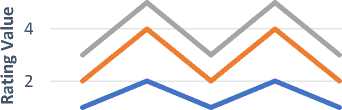
Illustrative Example 3 : Let us consider the rating vectors as shown in Fig. 2(a), which shows three rating vectors, V1, V2, and V3, corresponding to users U1, U2, and U3 respectively. Here, also note that V2 =2×V1 and V3 = 2×V1 +1; the traditional similarity measures such as PCC and COS result in inadequate values as explained earlier, while the proposed SMCC(U1, U2) = 3/5 =0.6 and Jaccard(U1,U2) = 5/8 = 0.625 (assuming | Iu ∪ Iv |= 8), therefore, JSMCC(U1, U2) will be 0.6 × 0.625 = 0.375.

Fig. 2(b) shows two flat rating vectors V1 and V2 = 5 × V1; For such vectors, PCC is not defined while the COS always results in 1 regardless of the differences between the rating vectors. Here, in this case, the proposed similarity measure provides zero similarity which is consistent with their conflicting nature.

item1 item2 item3 item4 item5

^^^^^wV1 ^^^^^e V2 ^^^^^в V3

(a)

ho 3

item1 item2 item3 item4 item5

—•—V1 —•— V2

(b)

• Fig.2. Illustrative rating vectors showing deceptive values of the PCC & COS (a) Scaling and shifting of rating vectors (b) Flat rating vectors.

While calculating the similarity between two users, the proposed similarity measure uses all the ratings given by two users in contrast to traditional measures that operate only on the co-rated items. Additionally, for commonly rated items, the proposed measure just compares the values of the rating pair to determine the interests of the two users for a particular item, which is quite an intuitive indicator of the similarities between the users. Finally, the empirical results on the different datasets (MovieLens-1M, 10M, and 20M) demonstrate the superiority of the proposed similarity measure against the traditional as well as state-of-art similarity measures in term of predictive accuracy, as explained in the experiment section.

IV. Experiments

There has been an ample amount of research in the area of recommender systems in nearly the last twenty-five years[23]. Therefore, an RS designer has a considerable range of algorithms available for developing his/her system and must find the most suitable approach based on his goals along with a few given constraints. Similarly, a researcher who proposes a new recommendation algorithm must evaluate the suggested approach against the various existing approaches by using some evaluation metric.

In both cases, academia and industry, one has to analyze the relative performance of the candidate algorithms by conducting some experiments. There are three primary types of experiments for evaluating recommender systems; offline experiments, user studies, and online experiments[47]. The later two types of experiments involve users whereas offline experiments require no communication with real users.

Offline experiments are typically the easiest to conduct and hence the most popular/accepted way of testing various recommendation approach[3]. An offline experiment is conducted with historical data, such as ratings, this pre-collected dataset must be chosen carefully to avoid any biases in handling users, items and ratings. Here, we have performed offline experiments on the standardized benchmark rating data sets from the

MovieLens website which is collected and made publicly available by the GroupLens research lab[48]. Table 8 summarizes these datasets briefly and more detailed description of the MovieLens datasets can be found in the article [49].

• A.    Experimental Design

We have employed the traditional user-based collaborative filtering (UBCF) algorithm with k-Nearest Neighbors(kNN) technique for validating the effectiveness of the proposed method against the baseline approaches. However, the proposed similarity measure takes the place of its counter component in the traditional UBCF as defined according to (6). Table 9 summarizes the details of the software and systems used for conducting all the experiments. The high-performance computing system is required to process the latest MovieLens-20M dataset because of its huge size which requires high memory requirement with more processing power. Furthermore, we have used the recently introduced framework, Collaborative Filtering 4 Java (CF4J)[50], for performing experiments. CF4J library has been designed to carry out collaborative filtering-based recommendation research experiments. It provides a parallelization framework specifically designed for CF and supports extensibility of the main functionalities. Simply, it has been developed to satisfy the needs of the researchers by providing access to any intermediate value generated during the recommendation process i.e. one can say that it is a “library developed from researchers to researchers”.

Table 8. The brief description of the datasets used

Dataset	Release Date	Brief Detail	Sparsity Level
MovieLens-1M	2/2003	•    1000,209 ratings from 6040 users on 3900 movies •    Each user has rated at least 20 movies.	1 - 1000,209 = 95.754 6040 ∗ 3900
MovieLens-10M	1/2009	•    10,000,054 ratings from 71567 users on 10681 movies •    Each user has rated at least 20 movies.	1 -   10000054   = 98.692 71567 ∗ 10681
MovieLens-20M	4/2015	•   20,000,263 ratings from 7138493 users on 27278 movies •    Each user has rated at least 20 movies.	1 -   20000263   = 99.470 138493 ∗ 27278

• B.    Evaluation metrics

Based on the general bibliography in the RSs research, accuracy is the most explored property for designing an RS. The fundamental rationale is that if a recommender system suggests more accurate recommendations then it will be preferred by users. Therefore, accuracy is considered as the most important goal for evaluating various candidate recommendation approaches[51]. Additionally, accuracy measurement is independent of the GUI provided by a recommender system. The offline experiments are well suited for simulating the accuracy measurement using the standardized benchmark datasets such as MovieLens. Here, we have evaluated the following two types of accuracy measures:

• •    Accuracy of predictions

• •    Accuracy of classifications

• a.    Measuring the accuracy of rating predictions

Let it is known that a user u has rated an item i with the rating r ui and a recommendation algorithm predicts this rating value as f^. Then, one can say that estimation error for this rating will be e_ui = f^ — r _ul i.e. the diffrence between the predicted score and the actual score. In order to compute the overall error of a system, for a given test set T of user-item pairs, Mean Absolute Error(MAE) and Root Mean Squared Error(RMSE) are the most popular metrics used in the literature as shown below by (7) and (8) respectively. MAE computes the average error while the RMSE sums up the squared errors, therefore, RMSE penalizes large error values.

MAE=1  ∑ |(rˆui-rui)|(7)

| ^T | ( u , i ) ∈ T

RMSE =1      (rˆ -r )2(8)

uiui

| ^T | ( u , i ) ∈ T

• b.    Measuring the accuracy of classifications

There are situations where it is not necessary to predict the actual rating values of items in order to provide recommendations to users but rather a recommender system tries to provide a list of items (topN items) that may be relevant or useful for users. As an illustration, when a user add a movie to the queue, Netflix[46] recommends a set of movies with respect to the added movie, here, the user is not concerned with the actual rating values of these suggested set of movies but rather the system correctly predicts that the user will add these movies to the queue.

Table 9. The details of the software and systems used.

High Performance Computing System	Intel(R) Xeon(R) Gold 6132(Skylake) 14 cores CPU@ 2.6GHz with 96GB RAM
Eclipse Java EE IDE	4.7.2 or higher
Java version (JRE)	Java 1.8 or higher
CF4J library version (framework)	1.1.1 or higher

In the recommender system scenario, the aim of a classification chore is to recognize the N most useful items for an active user. Therefore, we can use classic

Information Retrieval (IR) metrics to evaluate recommender systems. Precision and Recall are the most examined IR metrics, these metrics can be adapted to RSs without any difficulty in the following manner.

Precision : the proportion of top recommendations that are also relevant recommendations.

Recall : the proportion of all relevant recommendations that appear in top recommendations.

Formally, Let R(u) is the total number of recommended items to the user u, T(u) is the theoretical maximum possible number of relevant recommendations for that user u (which comes out to be the testing set actually), and β is the rating threshold to measure the relevancy. So the precision and recall may be defined using (9) and (10) respectively. Similar to the IR jargon, these metrics can also be defined using a 2 × 2

contingency table as shown in Table 10.

Table 10. Classification of all possible outcomes of a recommendation

	Recommended	Not Recommended
Preferred	True-Positive (tp)	False-Negative (fn)
Not preferred	False-Positive (fp)	True-Negative (tn)

V. Results and Discussions

The effectiveness of the proposed measure has been evaluated against the various baseline similarity measures, listed in Table 11 and explained earlier in the section of related work.

Table 11. The various baseline approaches compared with the proposed method

S.No.	Similarity Measure	Ref.
1	Pearson Correlation Coefficient (PCC)	[25]
2	Constrained Pearson Correlation Coefficient (CPCC)	[8]
3	Cosine Similarity (COS)	[14]
4	Adjusted Cosine Similarity (ACOS)	[40]
5	SRCC
6	Jaccard Index	[34]
7	Mean Squared Difference (MSD)	[8]
8	Jaccard Mean Squared Difference (JMSD)	[29]
9	Coverage-Jaccard-Mean Squared Difference (CJMSD)	[30]
10	Singularity-based similarity (SING)	[32]
11	Proximity-Impact-Popularity (PIP measure)	[27]

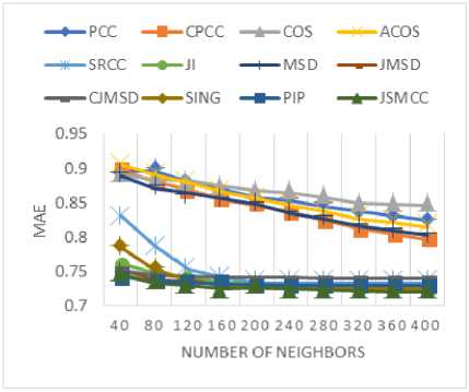
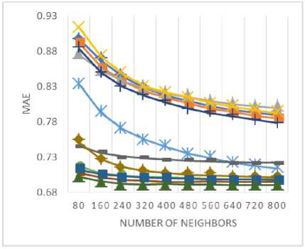
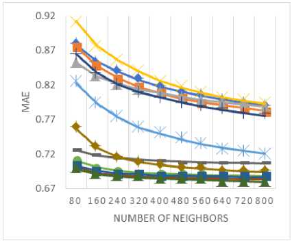
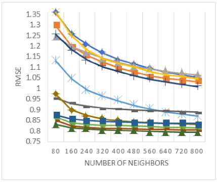
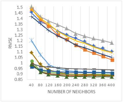
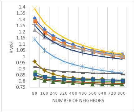
In order to determine the predictive accuracy, in terms of MAE and RMSE, we have used 80% of the rating data as training data and the remaining 20 % is used for testing purpose. Further, for each test user, 20% of his ratings are used for validation. Training and test data are chosen randomly in order to avoid any bias from the data selection. The values of MAE and RMSE are calculated for the proposed method along with various baseline approaches by varying the number of neighbors i.e. the neighborhood-size. MAE and RMSE values are compared for the proposed method against various baseline approaches in Fig. 3 and Fig. 4 respectively for (a) MovieLens-1M dataset (b) MovieLens-10M dataset, and (c) MovieLens-20M dataset.

(a)

(b)

(c)

Fig.3. The MAE values for (a) MovieLens-1M (b) MovieLens-10M (c) MovieLens-20M datasets.

As shown in Fig. 3(a)-(c), the empirically obtained values of MAE demonstrate that the proposed similarity measure results in lowers the MAE values against baseline approaches that indicates the better performance in terms of predictive accuracy. Likewise, the values of

RMSE, as shown in Fig. 4(a)-(c), represent the superiority of the proposed method against the various baseline measures. Based on the application at hand, either MAE or RMSE may be selected for evaluating the predictive accuracy. There is no decisive answer to this debate, research [52] compares and contrasts the relative advantages of MAE and RMSE metrics. Here, the proposed measure provides better results against the various baseline measures for both metrics, MAE and RMSE.

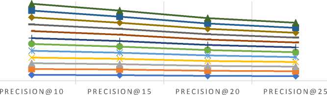
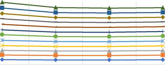
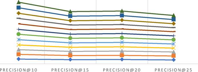
Furthermore, these predictive accuracy metrics such as MAE and RMSE are not enough for reflecting the true users’ experience, therefore, additional classification based metrics such as precision and recall are also used to evaluate the effectiveness of an algorithm [53]. We have also calculated the values of precision against the varying size of the recommended list i.e. top-N recommendations. Also, while evaluating precision values, the neighborhood size for each test user is kept to be fixed according to the datasets. Neighborhood-size is chosen in such a way that after the chosen size there is no significant improvement in the MAE/RMSE values for each dataset. Table 12 summarizes the different parameter values used for measuring precision values. Fig. 5 compares the precision values for different size of the recommended list for all three datasets (a) MovieLens-1M (b) MovieLens-10M (c) MovieLens-20M.

(b)

(a)

Table 12. The parameter involved in experimenting with the classification-based accuracy

	ML-1M	ML-10M	ML-20M
Test-Users %	20%
Test-Items %	20%
Rating Threshold (β)	4
Recommendation size	{10,15,20,25}
Neighborhood-Size	200	320	400

(c)

Fig.4. The RMSE values for (a) MovieLens-1M (b) MovieLens-10M (c) MovieLens-20M datasets.

As shown in Fig. 5 (a)-(c), the empirically obtained values of precision demonstrate that the proposed similarity measure provides better results for precision than the various baseline approaches, which shows the better performance in terms of classification accuracy. Based on the empirical results, we believe that the proposed method provides better results due to the following facts:

• •    It takes into account all the items rated by users, in contrast to the traditional measures which consider only commonly rated items (as the structural information between users are utilized using the Jaccard index)

• •    The actual rating values of all the commonly rated items are exploited to determine the proportion of items for which two users have shown similar rating pattern rather than finding any types of correlations (such as in PCC, CPCC) or angles (such as in COS) or other complex relation (such as in PIP, SING) between the rating vectors. This formulation is very simple and intuitive in nature.

  Precision

  
  

  Re call

  
  

^| { i ^e R ^{( u} )^: rm > P } I _     # tp

| R ( u )|         # tp + # fp

^| { i ^e R ^{( u} ) ^: rm > P } ^| _₌     # tP

| T ( u )|          # tp + # fn

VI. Conclusions

This article proposes a new similarity measure for neighborhood-based collaborative recommender systems. Finding similar users or items is an important step in collaborative filtering-based recommendation approaches. The proposed similarity measure is based on an adapted version of the simple matching coefficient together with the Jaccard index. Firstly, we have described a way to simulate the simple matching coefficient so that it can be applied to calculate the similarity between users or items, also, the structural information between rating vectors are also exploited using the Jaccard index.

Finally, several experiments have been performed for validating the effectiveness of the proposed measure against baseline methods. The empirical results demonstrate that the proposed method provides better predictive accuracy (in terms of MAE and RMSE metrics) and better classification accuracy (in terms of precision metric) than the baseline approaches. We believe that web-portals or e-commerce websites may utilize the proposed similarity measure into their existing recommender systems for improved accuracy because they have to just upgrade only the similarity measurement module. The effect of the proposed similarity measure on other RS goals such as diversity, coverage, etc. may be analyzed as the future task.

— ♦ — PCC  — ■ — CPCC —*— COS      ACOS —ж— SRCC —е—JI

4.8

3.8

2.8

1.8

0.8

-0.2

—I— MSD ■    JMSD ■    CJMSD    SING — ■ — PIP   —*—JSMCC

3.2

2.7

2.2

1.7

1.2

0.7

0.2

-0.3

3.5

2.5

1.5

0.5

(a)

PRECISION@10    PRECISION@15    PRECISION@20    PRECISION@25

(b)

(c)

Fig.5. The relative values of precision for varying size of the recommended list (a) MovieLens-1M (b) MovieLens-10M (c) MovieLens-20M datasets (Here, Precision values are shown on a scale while real values are between 0 and 1).