A note on migration perturbation and convergence rates to a steady state

Consider the Leslie population model, where y t is the vector of population size by age, that is, y it is the size of the population who are of age i at time t. The canonical Leslie matrix L is given by

L =

b 1

s 1

V0

• • Ц

0     •••

..     ...0

0   Sn-1

Aleksandra Lukina’s support from the Russian Foundation for Basic Research grant No 18-01-00551 is gratefully acknowledged.

Y-4.0

Here bi > 0, 1 < i < n, are age-specific fertility rates and 0 < si < 1, 1 < i < n — 1, are survival rates. Age-specific population growth from some initial distribution y0 is described by the equation yt+1 = Lyt.

If L is irreducible, the Perron-Frobenius theorem implies that a maximummodulus eigenvalue is real and positive. If in addition L is primitive, then there is a unique (real, positive) eigenvalue of maximum modulus, the Perron eigenvalue, whose eigenspace has dimension 1. The total population will grow or shrink according to whether the Perron eigenvalue is greater than or less than 1. These results may be found in any textbook on linear algebra or Markov Chains (see, for example, [1] , [2] ). Their applications to the Leslie population model may be found in [3] , section 4.5, or in [4] , section 5.

Our goal is to study the evolution of the age structure of the population; that is the evolution of the ratios y it /y jt . If L is irreducible and primitive with Perron eigenvalue A > 0, then taking x o = y o , x _t = A ^-1 Lx _{t -1} converges to a limit x ^∗ , a strictly positive member of the Perron eigenspace. Clearly x _it Jx j_t = y it /y jt , and so the age structure converges to a limit which is described by the vector x ^∗ . (The limit frequency distribution of ages is given by || x ^∗ || ₁ ^{- 1} x ^∗ , that is, x ^∗ divided by its l 1 norm.). In what follows we shall work with a normalized Leslie matrix. We will divide all the entries by the Perron eigenvalue in order to have a Leslie matrix with Perron eigenvalue equal to 1. This normalization leaves the Perron eigenspace unchanged, and forces the modulus of all eigenvalues other than the Perron eigenvalue to be less than 1. (This is what guarantees convergence of the x t to a nontrivial equilibrium.)

We assume that s i >  0 for all i < n. If some s k = 0, no one lives past age k, and the model can be truncated there. We also assume that b n >  0. The Leslie model is a model of a population in its reproductive years. Individuals may survive past age n , but they no longer contribute to population growth, and so the model does not track their behavior. These two assumptions guarantee that L is irreducible.

The Leslie matrix need not be primitive. For instance, if there are births only in even periods, there will be two real eigenvalues of maximal modulus. A positive age one birth rate is a sufficient condition for primitivity; however, this is not a good model for human populations. Fortunately, there is a sufficient condition for primitivity which is applicable to human populations, that the birth rate at two successive ages is positive, see [4] .

We consider the following thought experiment. The stationary age structure of a population is perturbed by an event: in- or out-migration, or a significant disease, that effects different ages differently. The age structure will be perturbed away from the stationary age structure. How long will it take for the system to come back to the steady state? We give answers to these questions, using tools developed to understand the behavior of random walks on graphs (see, for example, [5] ). Precisely, we provide lower and upper bounds for the time required to reach a given distance from the steady state.

This experiment has an important limitation. It assumes that the age-specific birth and death rates remain in the post-event population the same as they were in the pre-event population. We assume that emigrants have fertility and mortality patterns no different than those who remain; that with respect to fertility and mortality, immigrants behave just as does the home population; that the incidence of the disease is not correlated with fertility or with other co-morbidity factors. If the disease were to become endemic, as is expected to be the case with COVID-19, this will no longer be true.

Convergence times in the population models, when addressed at all, are described with asymptotic convergence rates. More precisely, the eventual rate of convergence to the stable age distribution is governed by the eigenvalue(s) with the second largest absolute magnitude. See, for example, [3] , equation (4.91) on p. 96, which implies that convergence to the steady state is asymptotically geometric, “at a rate at least as fast as log ρ”, where ρ is the damping ratio (the ratio of the largest eigenvalue to the second largest absolute eigenvalue). The damping ratio as the measure of “how quickly transient dynamics dissipate over time” is also mentioned in [6] . To the best of our knowledge, the tools we use in this paper have never been applied to studies of the short run dynamics of the Leslie population model.

• 1.    Convergence to a Steady State

Let L be the Leslie matrix (n x n) that is irreducible and primitive, and assume that the maximal Perron eigenvalue of L is 1 (otherwise, normalize). Denote a left Perron eigenvector of L by v 1 . A right Perron eigenvector of L consistently with what is above is denoted by x ^∗ .

First, the simplices S V = { x : v • x = a, x >  0 } are invariant under L for all a >  0.

Proposition 1. For any a >  0 the simplex S V is invariant under L.

Proof. If v • x = a and y = Lx, then v • y = v • Lx = v • x.       □

The implication of this is that all the dynamics live on S _α ^v where a = v • x ₀ . Instead of tracking population shares, it is easier to track motion on an invariant hyperplane, and rescale to get a probability distribution whenever we want.

We will assume for this section that v • x * = v • x ₀ . The basic linear algebra fact tells us

Proposition 2.

• (1)               || x t - x * || ^ 0 for any norm || • || on R ⁿ .

• 2.    Measuring System Fragility

The rest of the paper is devoted to estimating rates of this convergence in some specifically chosen norm.

One approach to fragility is to ask how long it takes to approach the steady state.

Define the l i -norm such that || x || i = Ei v i | x i | . Treating v as a positive measure, this could be thought of as a standard 1 1 norm on the measure space ( { 1,..., n } , v). This compares easily enough to the 1 1 norm (with respect to counting measure): min i v i || x || 1 < || x || V <  max i v i || x || 1 . Note that S i is the intersection of the non-negative orthant with the 1 1 -unit sphere. An important fact about these norms is the following:

Lemma 1. If x,y >  0 and || x || i = || y || i , then

• ^{| |x} - y || i = ²   52    v^ax i ^- y i ).

i : i i X i >i i y i

Proof. Let I = { i : v i x i > v i y i } . Then || x - y || i = E i _{c I} v i (x i - y i ) + E id c v i ⁽y i ^- x i ). AM E id v i x i + E id c v i x i = E id v i y i + E id c ^v i У i ^, so Ei c I c v i (y i - x i ) = Ei c I v i (x i - y i ). Substituting completes the proof.                                                                  □

Another fact we will need is that L does not increase v-distances.

Lemma 2. || Lx - Ly || ¹ _v ≤ || x - y || ¹ _v .

Proof.

^||Lx - LyH l = ^||L(x - y) || v

• <    || L • ( | x i - y i | , . . . , | x n - y n | ) || V since L is non-negative

• =    vL • ( | x i - y i | ,.. ., | x n - y n | )

• =    v • ( | x i - y i | , .. ., | x _n - y _n | ) since v is a Perron eigenvector =^{||x -} y || V .

□

From here through the end of this section we will work on S ₁ ^v , and take x * to be the Perron eigenvector in S i ; that is, || x * || V = 1. For an arbitrary initial condition x 0 , || x 0 || _v ^{- 1} x 0 is in S ₁ ^v , so it is easy to rescale the results.

Here are the key definitions. Let e k = (1/v k )e k where e ^ is the kth standard basis vector, i.e. e ^v _k are the vertices of the simplex S ₁ ^v . Two measures of a distance from the limit distribution are

• (2)                     d(t) = sup UL t y - x * || i ,

y∈S1v and

• ^{(3)                       d} ‘ ^(t) = ^{1 su}P ^||L t y ^- L t zH i .

• ² y,z E S V

All of the foregoing suprema are realized at the vertices of S ₁ ^v .

Lemma 3.

d(t) = max ||Ltei - x*||i, and

• ^d ‘ ^(t) = im k a l x ^||L t ^e k ^- L t e v || 1 .

Proof. The l _v ¹ norm is linear on S ₁ ^v . If z is not a vertex, it can be written as a convex combination of vertices, z = ^_fc а ^ е к . Then, using convexity of || x - y || _v in x, we get

||Ltz - x∗||v ≤∑︂αk||Ltevk-x∗||v k and so ||Ltz — x*||1 < max ||LteV — x*||1.

{ k:a k >0 }

Similarly, using convexity of || x — y || 1 in both arguments, one can prove the second statement of the lemma.                           □

The ob ject of interest, as we have phrased the fragility question, is the following time:

Definition 1. The recovery time for the norm 1 1 is

т ( e ) = min { t : d(t) <  e } ,

It is the first time the distance from x t to x ^∗ is guaranteed to be less than e no matter the initial condition. The goal is to estimate т ( e ) . One can imagine a similar recovery time for the distance d ^′ , but the next lemma makes obvious the connection.

Lemma 4. 1 d(t) <  d ' (t) <  d(t).

Proof. For the first inequality, note that x * = L t x * , so

d(t) = sup || L t y — L t x * || 1 <  sup || L t y — L t x * || 1 = 2d ' (t).

y ∈ S ₁ ^v                        y,z ∈ S ₁ ^v

The second inequality follows from the triangle inequality.

d ' ^(t) = 2 max ^||L t e k - L^ ^{11 1} <  ImT^L t e k - x * ^{11 1}

+ || x * — L t e V || V ) = d(t).

□

The distance d ' (t) is an operator norm on the subspace of R ⁿ which is orthogonal to v, with the i V -norm:

Lemma 5.

d - sup ^{||L t} x^{|| V d} ^ = x^O || x |I V

Proof. For any k and 1, v • (ek — eV) = 0 and ||eV — eV||V = 2. So i_ 1           t v _ -rt v 1              ||L x||v d (t)    2mkax ||Lek   Lel ||v < x:vuPo ||x||v .

In the other direction, there is no loss of generality in restricting the right hand side optimization to vectors x E Rn of l1-length 2. For any such vector x such that v • x = 0, let x+ = max{0, xi} and x— = max{0, —xi}, so that x = x+ — x—. Then x+,x- > 0 and v • x = 0 implies that l|x+llV = IIх-IlV = 1; that is, x+, x— E SV. Thus, sup ||L x|lv < 1 sup ||Lt(y — z)||V = d (t).

x:vx=0 H^x|| V ² y,z e S v

□

A key property of d ' (t) is that it is submultiplicative:

Lemma 6. d ' (s +1) <  d ' (s)d ' (t) .

Proof.

d ' (s + t) = |™ax I| L s ⁺ t e V - L+M Il V

= |max || L ^s (Le V — L^ V ) || V

• 2 k,l

• < d ' ^(s)|^max HL t e k ^— L t e v Il V

2 k,l

= d (s)d (t).

The inequality follows from lemma 5 and from the fact that v • (L t e V - L t e V ) = 0.                                                                               □

Here is an upper bound on т (e).

Theorem 1. For 5 < 1 and e < 5, т (e) < т (5)

log(e/2) log ^{( 5 )}

Proof. Fix 5 and e such that 0 < e < 5 <  1. Denote t * = т (5) so that d(t * ) = d(r (5)) < 5. According to lemmas 4 and 6 for any natural number k we get the following chain of inequalities:

d(kt * ) <  2d ' (kt * ) <  2(d ' (t * )) ^k <  2(d(t * )) ^k .

Choose k = Lt(е)/т(5)J = Lt(e)/t*J. For such k we have kt* < т(e), and therefore, d(kt*) > e. Then e < d(kt*) < 2(d(t*))k < 25k < 25T(e)/t* = 25т(е)/т(5).

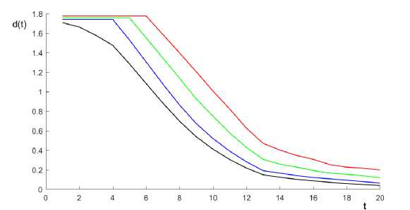
Figure 1. d ( t ) for different Leslie matrices specified below.

Taking logarithms, (recall that 5 <  1).

we get log(e/2) < ^T(j⁾ log 5, i.e. т (e) <  т (5) ^{log( e/ 2)} т (o)                             log 5

□

For example, if e < 1/2, т _х . (e) < (1 — log ₂ e^T x * (1/2). The content of the theorem is that, for e < 1 the recovery time grows like log e, i.e. once we are within the unit distance from x ^∗ the convergence is geometric. The l _v ¹ diameter of S ₁ ^v , however, is 2, so there is plenty of room for other types of behavior.

Figure 1 plots d(t) for four Leslie matrices that differ from each other only in the first row. n =20 and s i = 1 — 0.05i for 1 <  i <  19, Ь б = b 7 = b 8 = b 9 = 0.05, b io = bn = b i2 = 0.1, b i3 = b i4 = 0.05, b ₁₅ = b ₁₆ = 0.03, b 17 = 0.02, b ₁₈ = b ₁₉ = b ₂₀ = 0.01 in all 4 cases. The first matrix (corresponds to the black line in figure 1 is described by b 1 = 0.02, b ₂ = b ₃ = 0.03, b ₄ = b ₅ = 0.05; the second one (corresponds to the blue line) - b 1 = b ₂ = b ₃ = 0, b ₄ = b ₅ = 0.05; the third one (corresponds to the green line) — b 1 = b ₂ = Ь з = b 4 = 0, b 5 = 0.05; the fourth matrix (corresponds to the red line) — b 1 = b ₂ = b ₃ = b ₄ = b ₅ = 0 2 . The plots demonstrate the intuitive idea that adding more zeros to the first row (meaning that the youngest groups are not reproductive) makes convergence to a steady state slower. Moreover, the distance from a steady state measured as d(t) does not decrease for first several periods. The larger n is, the more space for such kind of behavior we have.

² These matrices require normalization to get the maximal eigenvalue equals 1.

Let us provide more intuition standing behind the figure 1 demonstration. From the Markov chains literature (see, for example, [7] , proposition 10.5), it is known that if a matrix is positive, then convergence to the steady state is geometric from the first period. A similar result might be proven for any primitive positive matrix that is not necessarily stochastic. 3 It is also known that convergence might be, on the contrary, very slow if a matrix under consideration contains a lot of zeros. As we show in figure 1 , the more zeros we have in the first row, the slower the system converges. That seems to be relevant for real demographic models because the more ages we consider, the more zeros we have in the first row (once we divide the population into more age-specific groups, more of them turn out to be non-reproductive).

Now let us lower-bound т (e).

Definition 2. The edge measure Q is defined on pairs of subsets of { 1,. .. , n } is defined to be

Q(A,B ) = E V i L ij x j .

j ∈ A, i ∈ B

Lemma 7. Let G be any set of indices, x ^∗ and v right and left Perron eigenvectors, respectively, of L corresponding to an eigenvalue λ. Then Q(G, G c ) = E^ c j V i L ij x j = E i _£ G E^ V i L ij x j = Q(G c , G).

Proof.

EE V i L ij x j+E E V i L ij x j	= E E V i L ij x j	= A ^2 V i x j
i ∈ G j ∈ G            i ∈ G j ∈ G c	i ∈ G j	i ∈ G
EE V i L ij x j + EE V i L ij x j	= EE V i L ij x j	= AEV j x j .
i ∈ Gj ∈ G           i ∈ G c j ∈ G Subtract to reach the conclusion.	i j ∈ G	j ∈ G □

There are several measures of flows across states in a non-negative linear system. One such is this:

Definition 3. For G c { 1,..., N } ,

ф(G) = QQGGl .

i ∈ G v i x i ^∗

Also define

Ф * =    min    Ф(G).

GE* V ii < 2

Theorem 2.

T (e) —

ε

2Ф

. ∗

Proof. For a given set G, define xG= /xi if i E G, and 0 otherwise,

G x x =       , where

|| x ^{G ||} V

HxGHV = Ev i ^x * . i ∈ G

Lemma 8. || Lx G - x ^G || V = 2Q(G,G ^c ).

Proof. From lemma 1 ,

H^Lx G - x ^G || V = ² EE v i ( L ij x j ^— x ^G ) .

i∈I j∈G where I = {i : ^j-eG LijxG — XG > 0}.

For i G G, ^j- _{e G} L ij x G <  ^j- L ij x j = X G , so i / I . If i / G, ^ jj e G L ij x G — 0 = X G . Thus I = G c , and

^||Lx G ^{— x G ||} V = ² ^^ v i ( L ij ^x G ^{— x} G )

i ∈ I j ∈ G

= 2 EE V i ( L ij x G — x G )

i ∈ G ^c j ∈ G

= 2 EE ViLij xG i∈Gc j∈G

= 2Q(G,G c ).

□

From this fact follows

|| Lx G — x ^G || V = 2Ф(G).

Per lemma 2, convoluting with L does not increase distance, so

\\ L t x G - x G || V <  ^ || L k x G - L ^{k - 1} x G || V <  t || Lx G - x G || V = 2tФ(G). k=1

Choose a set G such that ^ _{i e} G v i x * <  1/2. Then \\ x ^G — x * \\ V >  1. Therefore, using (4), we get

• ¹    < \\ x ^{G —} x * || v < \\ x ^{G —} L^txG\\V + \\L t x G ^— x *n v <

• < 2tФ(G) + \\L t x G — x * \\ V <  2tФ(G) + d(t).

The last inequality in this chain holds since \\ x ^G \\ V = 1.

Taking t — т (e) for which d(t) < e, we get

• 1    <  2т(e)Ф(G) + e.

• 3.    Recovery Times for the Leslie Matrix

Minimizing over G gives the result.

□

The preceding results apply to any n x n nonnegative, irreducible and primitive matrix. We have not yet taken advantage of the specific structure of the Leslie matrix in the previous section (all the results are true for any non-negative primitive matrix).

One can show that if the Perron eigenvalue of L is 1, the n4

—(11 — T

1 — b l — b 2 S 1

s 1 s 2

b 1

^{— b} 2 s i ^— • • • ^— b n - 1 s i • • • s n - 2 s l • • • s n - l

)

is a left Perron eigenvector. The last coefficient of v is equal to b n .

The right eigenvector must be normalized to S ₁ ^v . This requires dividing the coefficients of x by v • x. Denote the latter by n which is given by

П — n — (n — 1)b i — (n — 2)b 2 S 1 — (n — 3)b 3 S 1 S 2 — ... — b n - 1 S 1 • • • S n - 2 .

Define x * — n 1 x.

Theorem 1 (that does not involve the Leslie structure explicitly) is useful in the following sense: it allows to give a prior judgment whether perturbation of the population distribution is significant or not. Suppose a perturbed population distribution vector stays inside the simplex S ₁ ^v . In that case, we know that convergence back to the steady state will be geometric, so crucial changes in the population structure are impossible even in the middle run.

However, as we saw in the figure 1 , it might be the case that convergence is not any close to geometric in the short run (more precisely, d(t) may not decrease for several periods), and geometric convergence kicks off later. In such cases, it might be necessary to lower-bound a recovery time. Knowing entries of the Leslie matrix and shuffling different subsets G of { 1,..., n } such that ^_{i E} G v i x * <  1/2 one may use theorem 2 to give a lower bound for a recovery time for any given value of ε.