A Novel Application of Artificial Neural Network for the Solution of Inverse Kinematics Controls of Robotic Manipulators

Published Online August 2012 in MECS

A manipulating arm of a manipulator are consists of links that are connected by joints. These joints are either rotational or prismatic, i.e. change their length and thus providing additional degrees of freedom. The position of the manipulators end-effectors is fully described by its joint angles and joint offset by giving the knowledge of length of all rigid links. Therefore, to developing control mechanism for the robot arms, we have to understand the relationship between the actuators. If the position or angle of each joint known to us, then we can calculate the position of its end effectors using mathematical relationship (trigonometric) and this process is known as Forward Kinematics. Alternative relationship to forward kinematics is known as Inverse Kinematics [1-3].

In comparison to forward kinematics, understanding inverse kinematics is difficult. In forward kinematics, real systems are under-constrained, for a given goal position, there could be infinite solutions. In briefly, for inverse kinematics, many different joint configurations could lead to the same end point. Therefore, the inverse kinematics solution is a major problem in robotic research area. For solving the inverse kinematics, many traditional methods such as algebraic, geometric and iterative solutions are adopted. These methods are time consuming, high computational cost and suffer from numerical problems. These demerits of the mathematical models enthusiastic researchers for applying intelligent systems such as Fuzzy Logic, Neural Network etc. for solving inverse kinematics[4-6].

From the literature review, it was found that many methods have been proposed to solve the inverse kinematics instead of traditional computational methods. Utilization of Artificial Neural Network (ANN), Fuzzy

Logic System and Evolutionary computation algorithms for solving the inverse kinematics was reported in literatures. For ANN, presence of hidden layers, for fuzzy logic, number of rule bases and for evolutionary methods, the complex algorithms are associated with high complexity and high computational load. These methods may give good results, however these methods are difficult to implemented hardware. To overcome this problem, Functional Link Artificial Neural Network (FLANN) was applied to solve the inverse kinematics after successfully implemented in other complex engineering problem [5-7].

• II.    Introduction to Manipulator

According to robotic research, an industrial robot is comprised of a robot manipulator, power supply, and controllers. In general, robot manipulators are created from a sequence of link and joint combinations. The links are the rigid members connecting the joints, or axes. The axes are the movable components of the robotic manipulator that cause relative motion between adjoining links. Therefore, manipulators deal with inverse kinematics and direct kinematics. Manipulator control problem can be identified into two special areas and that are kinematics control (the coordination of the links of kinematics chain to produce desire motion of the robot), and dynamic control (driving the actuator of the mechanism to follow the commanded position velocities). Most of the problems are dealing with kinematics control and this paper highlighted one application on inverses kinematics hence dynamic control not discussed here. The details of inverse kinematics were briefly discussed as follows [2-4].

• A.    Introduction to Inverse-Kinematics

Inverse kinematics refers to the use of the kinematics equations of a robot to determine the joint parameters that provide a desired position of the end-effectors . Specification of the movement of a robot so that its endeffectors achieves a desired task is known as motion planning. Inverse kinematics transforms the motion plan into joint actuator trajectories for the robot. The Inverse Kinematics is the opposite problem as compared to the forward kinematics. The set of joint variables when added that give rise to a particular end effectors or tool piece pose. Kinematics is the study of motion [3-4]. In this proposed work, solution of inverse kinematics of 3R and 2R planar manipulator is discussed. Fig.1 represent the schematic diagram of both 3R and 2R planar manipulator

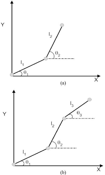
Fig.1: (a) Two DOF Manipulator (b) Three DOF Manipulator

• B.    Mathematical Solution to 3R Planar:

From the basic trigonometric, the position and orientation of the end effectors can be written in terms of the joint coordinate, the direct kinematics equations are:

x = l j cos 0 + l ₂ cos( 0 + 0 ₂) + l ₃ cos( 0 + 0 ₂ + 0 ₃) (1) y = l_x sin 0 + l ₂ sin ( 0 + 0 ₂) + l₃ sin ( 0 + 0 ₂ + 0 ₃) (2)

Ф = 0 + 0 + 0                        (3)

y - 1 ₃ sin( ^ ) = 1 1 sin 0 1 + 1 ₂ sin ( 0 1 + 0 2 )        (5)

Replacing x / = x - l₃ cos( q ), y / = y — l₃sin( Q ) regrouping and add each term of equation, we get a single non-linear equation in 0 1 .

(-2 1 1 x^! cos 5 ₁) + (-2 1 1 y / sin 5 ₁) + ( x /2 + y /2 + 1 ²1 - 1 22) = 0 (6)

Solving to equation (6) as consider it a single nonlinear equation (P Cos a + Q Sin a + R =0) the 9 ₁ becomes

5 = Y + o cos 1

x11 + y/2 + 121 - 122 21Jx/2 + y/2

where

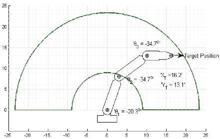
Fig.2: Solution to 3-R Planner using MATLB-GUI

Y = a tan 2

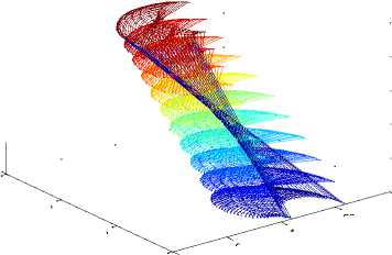
co-ordinates generated for all theta1,theta2 and theta3 combinations using forward kinematics fo

There are two solution for 9 ₁, as о = ± 1, hence the tow solutions are formed

Cos (5 + 5) =

x/ - 1[ cos 5

l ₂

/

Sin (5 + 5) = —

-1] sin 5

l 2

These two equations (9 and 10) are helping to solve the 9 2 using atan2 and we get the value of 9 2

(a)

5 = a tan 2

y / - 1X sin 5

x/ - 1X cos 5

l 2

l 2

- 0 1 (11)

Squaring the equations (4) and (5) and using Cos (a +

b) formulae, we get the solution for 9 1

5 = a tan 2 {(kxy / - k^x/), (kxx/ - k^y /)}  (12)

where k1=11+ 12cos92, k2=12sin92, x=x - 13cos(^), y= y- l3sin92. Then the solution of 92

0.8

0.6

0.4

0.2

Y Axis

X Axis

0   -10

5, = a tan 2 (sin 5,, cos 5,)

Cos 5

x2 + y 2 - 121 - 12 2

2ll

Sin5 = 7± (1 - cos 5)

Solution for 9 3

5з = ^ - (51 + 52)

Using the above expressions (12, 14, 16), a solution for 3-R planner is developed using MATLAB Graphical user interface (GUI). Fig. 2 represents the solution for 3-R Planner using MATLAB GUI. Fig. 3 represents the Simulation result for 3R planner using MATLAB GUI.

(b)

(c)

(d)

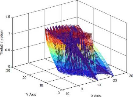
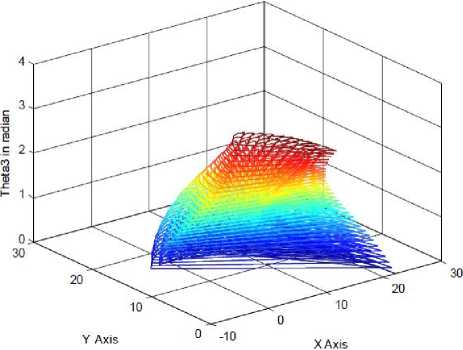
Fig.3: Simulation result of 3-R Planner using MATLB-GUI

(a) Workspace of the three-link planner

(b) Surface plot of the three-link planner ( G 1 with X and Y coordinates)

(c) Surface plot of the three-link planner ( G 2 with X and Y coordinates)

(d) Surface plot of the three-link planner ( G 3 with X and Y coordinates)

The algorithms of both the techniques were discussed as follows:

Application of Multi Layer Perceptron based solution to Inverse Kinematics

Stepwise algorithm of MLP system is represented as following manner:

Step 1: Select the total number of layers m, the number n i (i=1,2, . . . ,m-1 )of the neurons in each hidden layer and an error tolerance parameter 0.

Step 2: Randomly select the initial values of the weight vectors w^mi , j , for i=1,2, . . . ni and m=2 (number of layers).

Step 3(Initialization): All the weights w ^m i , j were initialized to random number and given as w ^m i , j (0)

w ^m i , j ←w ^m i , j (0)                            (24)

Step 4 (Calculation of the neural outputs):

Mathematical Solution to 2R Planar:

Similar to 3-R Planner, forward kinematic equations for 2-R planner are x = lj cos ^ + 12 cos (0 + 02 )

y = 1X sin 0 + 12 sin (0 + 02)

Squaring the equations (17) and (18) and add these equations we will get x + y = 121 +122 + 2Цг cos(0 + 02 )

m 1

I a i , j = ( W i , j ) x X_k

• 1         l 2 x m

L y j = ( W i , j ) x a j

Step 5 (Calculation of the output error):

The error was calculated as ej = dj - yj . It may be seen that the network produces a scalar output.

Step 6 (Calculation of the derivative of network output of each layer):

For hidden layer ( m =1)

The derivative of activation function of hidden layer can be represented as

Solving the equation (19), we will get

Cos 0

x ² + y ² - 1 ²1 - 1 2 2

2 ll

and Sin 0 = -J ± (1 — cos 0 ₂ )

•1          d f (n') = T dn

(     1

к 1 + exp ^- -

1      )

x --------

( 1 + exp ^{- n} J

¹ -к

1 + exp ^{- n} J

(1 - a ™ , j )( a m, , j )

Hence we will find the solution for G 1 , G ₂ as follows: 0 = a tan 2 { ( y , x ), ( k , k ₂) }                (22)

0₂ = a tan 2 (sin 0 ₂, cos 0 ₂)               (23)

For output layer ( m =2)

The derivative of activation function of output layer can be represented as

•2         d f (n2) = — (n) = 1 dn

• III.    Application of Artificial Neural Network for Solution of Inverse Kinematics

In this proposed work, the inverse kinematics problem was simulated using Artificial Neural Network (ANN) methodologies [8-12]. Two type of ANN methods, Multi-Layered Perceptron (MLP) and Functional Link Artificial Neural Network (FLANN) [13-16] were used to solve Inverse Kinematics problem.

Step 7 (Back-propagation of error by sensitivities at each layer):

Back-propagation of error by sensitivities at each layer was calculated as follows:

For output layer ( m =2)

• ²                                • ²

s ² j =- 2 F ( n ² )( — j - y j ) = - 2 f ( n ²) x ( e j )   (28)

For hidden layer (m=1)

5\ = F ( n 2 )( w \j)T s 2J =

(1 - a\j\ a V j )        0         -         0

0        (1 - a 2 i,j )( a J  -          0

where k is the time index and α is the momentum parameter.

Step 8: If error ≤ ε (0 . 01) then go to Step 8 otherwise, go to Step 3.

Fig.4 represents the flowchart of the proposed FLANN based architecture.

0              0         -   (1 - a ¹ J a ¹ „„ j )

2 T 2

X ( w i,j ) s j

Step 8 (Updating the weight vectors):

The weight matrices are updated next using the following relationship

w2 i, j (new) = w2 i, j (old) + ns 2 j (a1 i, j ) T w1 i, j (new) = w1 i, j (old) + ns1 j

Step 9:

If error < s (0.01) then go to Step 10, otherwise go to

Step 3.

Step 10:

After the learning is completed, the weights were fixed and the network can be used for testing.

Application of Functional Link Artificial Neural based solution to Inverse Kinematics

Step 1: Initialize the inputs as X and Y coordinates and the desired output of the manipulator.

Step 2: Randomly select the initial values of the weight vectors w_i , for i = 1, 2, . . . l , where “ i ” is the number of functional elements.

Step 3 (Initialization): All the weights w i were initialized to random number and given as w i (0)

w i ← w i (0)                               (31)

Step 4 (Produce functional block): For FLANN the functional block is made as follows:

Xi = [1, x1, sin(πx1), cos(πx1), x2, sin(πx2), cos(πx2) . . .]

Step 5 (Calculation of the system outputs): For functional based neural network models, the output was calculated as follows:

(^

Oj = tanh ^ w, x Xj

1 1:1       J

Step 6 (Calculation of the output error): The error was calculated as e_i = d_i - O_i . It may be seen that the network produces a scalar output.

Step 7 (Updating the weight vectors): The weight matrixes are updated next using the following relationship:

w i ( k + 1) = w i ( k ) + αe i ( k ) X i ( k ) (34)

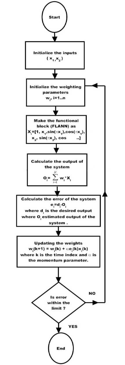
Fig. 4: Flowchart of FLANN based Inverse Kinematic elucidation

• IV.    Result and Disscussion

To solve the Inverse Kinematics, here two types of ANN methodologies (MLP and FLANN) are adopted. This entire simulation is done using the MATLAB simulation environment. This proposed system was simulated with the help of Pentium Core due Processor 3.2 GHz CPU, 2 GB based RAM and 300 GB storage capacity based Personal Computer. Using the mathematical relationship, both the model (MLP and FLANN) were applied to predict the joint angles of the manipulator using inverse kinematics equation. Let the analysis of MLP is discuss first. For 2D planner, 2-20-2 based MLP structure was chosen, where two number of inputs ( CARTESIAN COORDINATE (X AND Y)), twenty numbers of hidden nodes in the hidden-layer and two number of output in the systems. Fig. 5 represents the Mean square error plot for 9 1 , where Fig. 6 represents the testing result of the model. The mean square errors of the proposed system were calculated as follows:

1 Г

MSE = I ^ Desvredi - Eastimatedi I n к i=1                               )

Where n is the total number of samples of the proposed system.

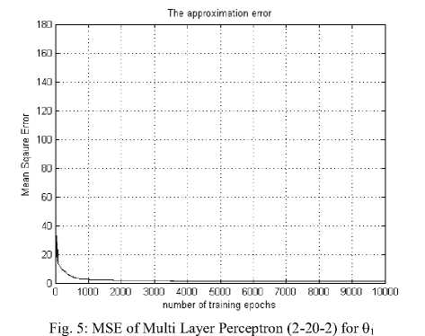
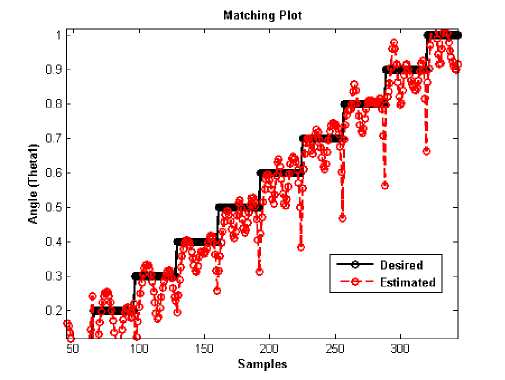
Fig. 6: Testing Result of Multi Layer Perceptron (2-20-2) for 9 1

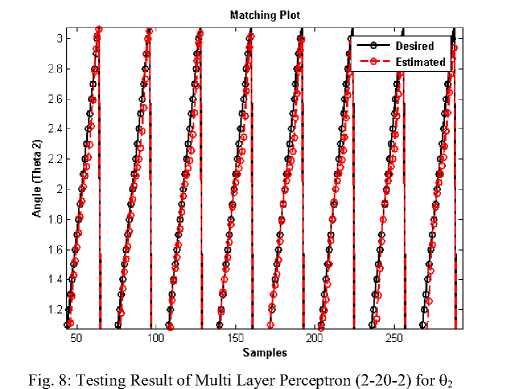
Fig. 7 represents the Mean square error plot of MLP system for 9 2 , where Fig. 8 represents the testing result of the model.

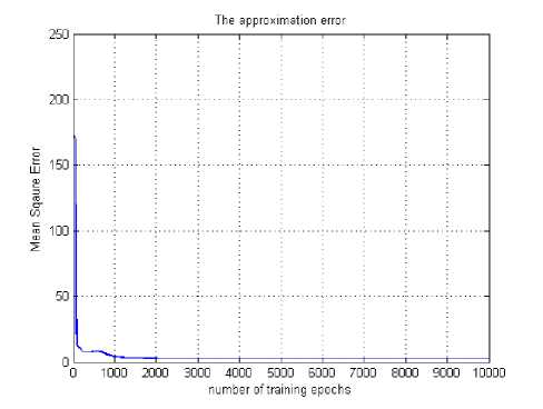
Fig. 7: MSE of Multi Layer Perceptron (2-20-2) for 9 2

Like MLP, for 2D planner, 2-7-2 based FLANN structure was chosen, where two number of inputs (CARTESIAN COORDINATES), seven numbers of hidden nodes in the hidden-layer (seven number of expansion) and two number of output in the systems. Fig. 9 represents the Mean square error plot for 9 1 , where Fig. 10 represents the testing result of the model.

The approximation error

0 Г г i i i i I i i i ---------

0    1000 2000 3000 4000   5000 6000 7000 8000 9000 10000

number of training epochs

Fig. 9: MSE of FLANN (2-7-2) for 9 i

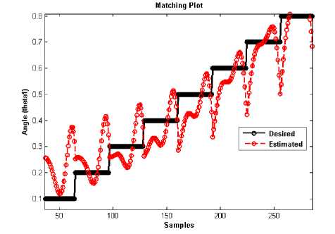
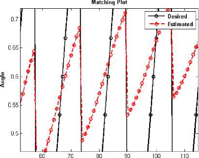
Fig. 10: Testing Result of FLANN (2-7-2) for θ 1

Fig. 11 represents the Mean square error plot of FLANN system or θ 2 , where Fig. 12 represents the testing result of the model.

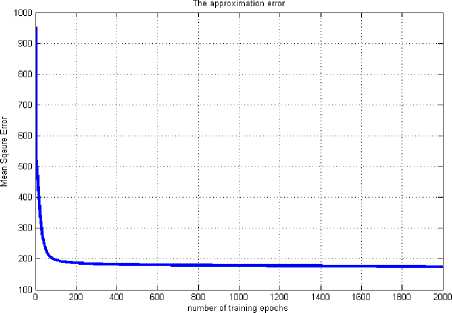
Fig. 11: MSE of FLANN (2-7-2) for θ 2

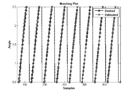
Fig. 12: Testing Result of FLANN (2-7-2) for θ 2

Result analysis of 3-D Planner

Similar to 2-D Planner, Using the mathematical relationship, both the model (MLP and FLANN) were applied to predict the joint angles of the manipulator using inverse kinematics equation. Let the analysis of MLP is discuss first. For 3D planner, 2-20-3 based MLP structure was chosen, where two number of inputs (CARTESIAN COORDINATES), twenty numbers of hidden nodes in the hidden-layer and three number of output in the systems. Fig. 13 represents the Mean square error plot for θ1, where Fig. 14 represents the testing result of the model.

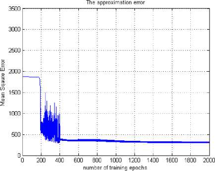
Fig. 13: MSE of Multi Layer Perceptron (2-20-3) for θ 1

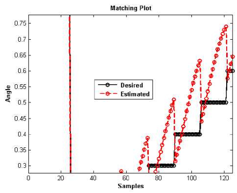
Fig. 14: Testing Result of Multi Layer Perceptron (2-20-3) for θ 1

Fig. 15 represents the Mean square error plot of MLP system for θ ₂, where Fig. 16 represents the testing result of the model.

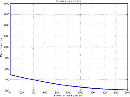
Fig. 15: MSE of Multi Layer Perceptron (2-20-3) for θ 2

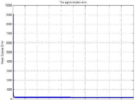
Fig. 17: represents the Mean square error plot of MLP system for θ 3 , where Fig. 18 represents the testing result of the model.

200     400     000 ООО 1000    1200    1400    1000    1000    2000

number of training epochs

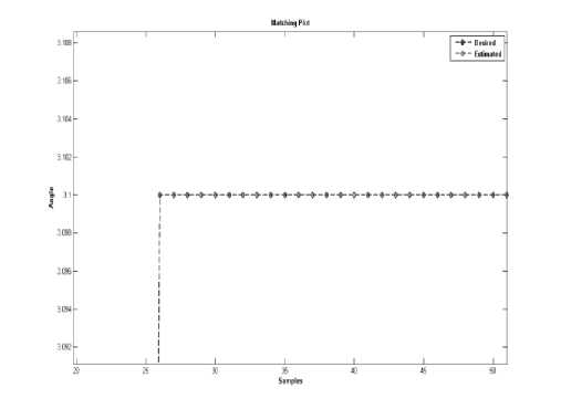
Fig.18: Testing Result of Multi Layer Perceptron (2-20-3) for θ 3

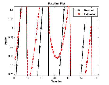
Fig. 16: Testing Result of Multi Layer Perceptron (2-20-3) for θ 2

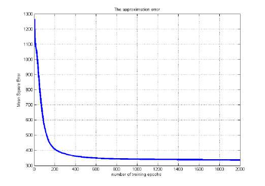
Fig. 19: MSE of FLANN (2-7-3) for θ 1

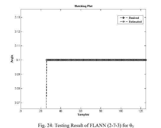
Like MLP, for 3D planner, 2-7-3 based FLANN structure was chosen, where two number of inputs (CARTESIAN COORDINATES), seven numbers of hidden nodes in the hidden-layer (seven number of expansion) and three number of output in the systems. Fig. 19 represents the Mean square error plot for θ 1 , where Fig. 20 represents the testing result of the model.

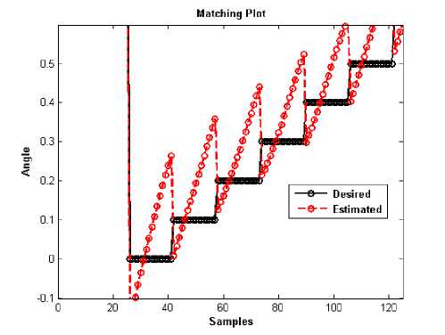
Fig. 20: Testing Result of FLANN (2-7-3) for θ 1

Fig. 21 represents the Mean square error plot of FLANN system for θ ₂, where Fig. 22 represents the testing result of the model.

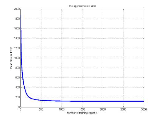
Fig. 21: MSE of FLANN (2-7-3) for θ 2

system. The performances of the both models were compared by considering the CPU time.

Table 1: Performance analysis of the proposed model (MLP and FLANN)

Type of the structure	Architecture	Applications	CPU time in sec.
2-20-2	MLP	2-D Planner	15.2389
2-7-2	FLANN	2-D Planner	2.8411
2-20-3	MLP	3-D Planner	46.2173
2-7-3	FLANN	3-D Planner	8.2745

Samples

Fig. 22: Testing Result of FLANN (2-7-3) for θ 2

• V.    Conclusion

Fig. 23 represents the Mean square error plot of FLANN system for θ 3 , where Fig. 24 represents the testing result of the model.

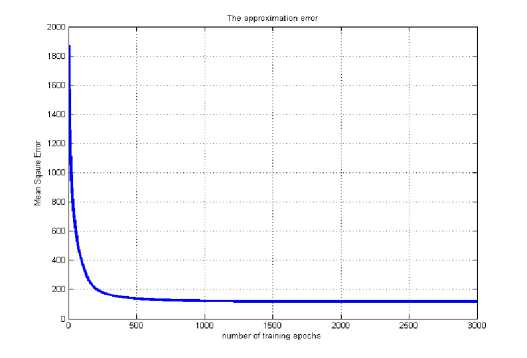
Fig. 23: MSE of FLANN (2-7-3) for θ 3

To find the performance analysis of the both the proposed model, CPU time comparison was done. Table 1 represents the performance analysis of the proposed

In this proposed research work two types of ANN architecture were applied to solve a complex problem of Industrial Manipulator. In this problem MLP and FLANN models were successfully implemented for both 2-D and 3-D planar. Categorically the proposed research problem can be alienated into two steps;

In the first step, using MATLAB Simulation Environment, the mathematical solution for both 2-D and 3-D Planar were executed and summarized. It was observed that the mathematical models are very complex with large number of computational load (Multiplication, Addition, Subtraction, Division) and therefore to reduce this complexity, here MLP and FLANN systems were proposed.

After the simulation it was found that the FLANN structure has very less CPU-time, with comparison to MLP system. It was observed that the proposed FLANN system was 5 times faster than MLP system and it can easily be implemented in hardware.

Acknowledgement

The authors like to thank to Prof. (Dr.) Radhakanta Mishra , Chairman of Eastern Academy of Science and Technology for his guidance, valuable comments, giving research facilities and words of encouragement. His motivation and guidance helped to improve the clarity of this paper.