A Novel Cat Swarm Optimization Algorithm for Unconstrained Optimization Problems

Published Online October 2013 in MECS

Optimization, Evolutionary Algorithms of birds [2], Bee Colony Optimization (BCO) which imitates the behavior of bees [3] and the recent finding, Cat Swarm Optimization (CSO) which imitates the behavior of cats [4].

By simulating the behavior of cats and modeling into two modes, CSO can solve the optimization problems. In the cases of functions optimization, CSO is one of the best algorithms to find the global solution. In comparison with other heuristic algorithms such as PSO and PSO with weighting factor [7], CSO usually achieves better result. But, because of algorithm complexity, solving the problems and finding the optimal solution may take a long process time and sometimes much iteration is needed.

So in this article, we propose an improved CSO in order to achieve the high convergence accuracy in less iteration. First we use an adaptive inertia weight and adaptive acceleration coefficient. So, the new velocity update equation will be computed in an adaptive formula. Then, our aim is to consider the effect of previous/next steps in order to calculate the current position. So by using a factor namely ‘Forgetting Factor’, information values of steps will be different. Finally, we use an average form of position update equation composing new velocity and position information. Experimental results for standard optimization benchmarks indicate that the proposed algorithm rather than pure CSO can improve performance on finding the best global solution and achieves better accuracy level of convergence in less iteration.

The rest of article is organized as follows: in section 2 basic of CSO is reviewed in two phases. Section 3 introduces new CSO with adaptive parameters and novel position equation. Experimental results and comparison of proposed CSO with pure are discussed in last section.

P i =

| SSE i - SSE max|

SSE max

- SSE_min

If the goal of the fitness function is to find the minimum solution, FS b = FS max , otherwise FS b = FS min

• II.    Cat Swarm Optimization

• 2.1    Seeking Mode

Cat Swarm Optimization is a new optimization algorithm in the field of swarm intelligence [4]. The CSO algorithm models the behavior of cats into two modes: ‘Seeking mode’ and ‘Tracing mode’. Swarm is made of initial population composed of particles to search in the solution space. For example, we can simulate birds, ants and bees and create Particle swarm optimization, Ant colony optimization and Bee colony optimization respectively. Here, in CSO, we use cats as particles for solving the problems.

In CSO, every cat has its own position composed of D dimensions, velocities for each dimension, a fitness value, which represents the accommodation of the cat to the fitness function, and a flag to identify whether the cat is in seeking mode or tracing mode. The final solution would be the best position of one of the cats. The CSO keeps the best solution until it reaches the end of the iterations [5].

Cat Swarm Optimization algorithm has two modes in order to solve the problems which are described below:

For modeling the behavior of cats in resting time and being-alert, we use the seeking mode. This mode is a time for thinking and deciding about next move. This mode has four main parameters which are mentioned as follow: seeking memory pool (SMP), seeking range of the selected dimension (SRD), counts of dimension to change (CDC) and self-position consideration (SPC) [4].

The process of seeking mode is describes as follow:

Step1: Make j copies of the present position of catk, where j = SMP. If the value of SPC is true, let j = (SMP-1), then retain the present position as one of the candidates.

Step2: For each copy, according to CDC, randomly plus or minus SRD percent the present values and replace the old ones.

Step3: Calculate the fitness values (FS) of all candidate points.

Step4: If all FS are not exactly equal, calculate the selecting probability of each candidate point by (1), otherwise set all the selecting probability of each candidate point be 1.

Step5: Randomly pick the point to move to from the candidate points, and replace the position of catk.

• 2.2    Tracing Mode

Tracing mode is the second mode of algorithm. In this mode, cats desire to trace targets and foods. The process of tracing mode can be described as follow:

Step1: Update the velocities for every dimension according to (2).

Step2: Check if the velocities are in the range of maximum velocity. In case the new velocity is overrange, it is set equal to the limit.

Vк,d =Vк,d+r1^c1 (Xbest,d -Хк,d )                 (2)

Step 3: Update the position of cat k according to (3).

_Xк,d =Xк,d +Vк,d                                (3)

X best,d is the position of the cat, who has the best fitness value, X k,d is the position of cat k , c 1 is an acceleration coefficient for extending the velocity of the cat to move in the solution space and usually is equal to 2.05 and r₁ is a random value uniformly generated in the range of [0,1].

• 2.3    Core Description of CSO

In order to combine the two modes into the algorithm, we define a mixture ratio (MR) which indicates the rate of mixing of seeking mode and tracing mode. This parameter decides how many cats will be moved into seeking mode process. For example, if the population size is 50 and the MR parameter is equal to 0.7, there should be 50×0.7=35 cats move to seeking mode and 15 remaining cats move to tracing mode in this iteration [9]. We summarized the CSO algorithm below:

First of all, we create N cats and initialize the positions, velocities and the flags for cats. (*) According to the fitness function, evaluate the fitness value of the each cat and keep the best cat into memory (X best ). In next step, according to cat’s flag, apply cat to the seeking mode or tracing mode process. After finishing the related process, re-pick the number of cats and set them into seeking mode or tracing mode according to MR parameter. At the end, check the termination condition, if satisfied, terminate the program, and otherwise go to (*) ^[9].

• III.    Modified Cat Swarm Optimization

• 3.1    Using Adaptive Parameters

The tracing mode of CSO has two equations: velocity update equation and position update equation. For reaching to an adaptive CSO, we change some of the parameters in velocity equation. Also for computing the current position of cats, we consider the information of previous and next dimensions by using a special factor and then we achieve a new dynamic position update equation. We describe the proposed algorithm in two parts.

In the proposed algorithm, we add an adaptive inertia weight to the velocity equation which is updated in each dimension. By using this parameter, we make a balance between global and local search ability. A large inertia weight facilitates a global search while a small inertia weigh facilitates a local search. First we use a large value and it will be reduced gradually to the least value by using (4).

W(i) = W + ⁽ⁱ -X ^{- і)} (4) 2×imax

Equation (4) indicates that the inertia weight will be updated adaptively, where W_s is the starting weight, i_max is the maximum dimension of benchmark and i is the current dimension. So the maximum inertia weight happens in the first dimension of the each iteration and it will be updated decreasingly in every dimension. In the proposed algorithm W s is equal to 0.6. Also, c 1 is an acceleration coefficient for extending the velocity of the cat to move in the solution space. This parameter is a constant value and is usually equal to 2.05, but we use an adaptive formula to update it by (5).

• - ⁽ⁱ max - і)

• 3.2    New Dynamic Position Update Equation

C(i) = Cs -                                  (5)

2×i

Equation (5) demonstrates that the adaptive acceleration coefficient will be gradually increased in every dimension and the maximum value happens in the last dimension. Here C s is equal to 2.05. By using these two adaptive parameters, we change the velocity update equation for each cat to a new form describing in (6).

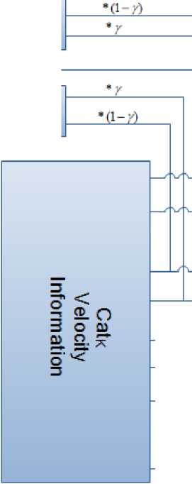
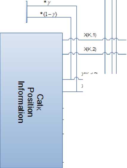
In this part, we change the position update equation to a new form. In the pure CSO, the position of cat is including of current information of velocity and position. Sometimes in many cases, using of previous information in order to estimate the current position is useful. Also, taking the advantages of next information can be appropriate information for updating the cat’s position. So we use the two previous/next dimensions information of velocity and position by applying a new factor which is called ‘Forgetting factor’. By this factor, the values of previous and next steps will be different. So the information value for first previous/next step is higher than second previous/next step. It means that the influence of previous/next step is more important than previous/next second step. New position update equation is described by (7).

In the proposed algorithm, γ is the forgetting factor and is equal to 0.6 (It is necessary to use γ > 0.5). This new position update equation is composing two new dynamic terms, average position information and average velocity information. Here, we use the current and the average information of first and second previous/next dimensions for both velocity and position by applying a forgetting factor (γ). Figure 1 shows the process of position updating for cat k .

^Xk,^{d =} 2 ^[ +(Velocity Information) ^{]             (7)}

Position Information = X , +

(γ×(X к , d+1 )+(1-γ)×(X к , d+2 )) 2 ⁺

(γ×(X к , d-1 )+(1-γ)×(X к , d-2 ))

Velocity Information = V , +

(γ× (V к , d+1 )+(1-γ)×(V к , d+2 )) 2 ⁺

(γ× (V к , d-1 ) + (1 - γ) × (V к , d-2 ))

Vк,d = W(d) × Vк,d+r1 × C(d)

× (Xbest,d-Xк,d )       (6)

Velocity Information

Average Processing

Average Processing

V(K,1)

V(K,2)

VfK.d-2}

VfK.d-1)

V(K,d)

V{K,d+1>

V(K,d+2)

VfK.m)

Average Processing

У

Position Information

Average Processing

4K,d)

Average Processing

^K,d-2/

XK.d-1)

*K.d)

XK.d+1)

XK.d+2)

XK.m)

Fig. 1: Process of position updating for cat k

IV. Experiment and Result In this paper, simulation experiments are conducted in GCC compiler on an Intel Core 2 Duo at 2.53GHz with 4G real memory. Our aim is to find the optimal	Table 1: Parameters settings for pure CSO
	Parameter	Range or Value
	SMP	5
	SRD	20%
solution of the benchmarks and find the minimum.	CDC	80%
Rastrigrin, Griewank, Ackley, Axis parallel, Trid10 and Zakharov are six test functions used in this work. In Table 1 and Table 2 we determine the parameter values of the pure CSO and Adaptive Dynamic CSO	MR	2%
	C 1	2.05
	R 1	[0,1]
respectively. The limitation range of six test functions is mentioned in Table 3.

Table 2: parameter settings for adaptive dynamic CSO

Parameter	Range or Value
SMP	5
SRD	20%
CDC	80%
MR	2%
R 1	[0,1]
Starting Adaptive Acceleration Coefficient (C s )	2.05
Starting Adaptive Inertia Weight (W s )	0.6
Forgetting Factor (γ)	0.6

Table 3: Limitation range of benchmark functions

Function Name	Limitation Range	Minimum	Population Size
Rastrigin	[2.56,5.12]	0	160
Griewank	[300,600]	0	160
Ackley	[-32.678,32.678]	0	160
Axis Parallel	[-5.12,5.12]	0	160
Zakharov	[-100,100]	0	160
Trid10	[-5,10]	-200	160

Table 4: Experimental results of Rastrigin function

Algorithm	Average Solution	Best Solution	Best Iteration
Pure CSO	26.64208	1.161127	2000
Adaptive Dynamic CSO	18.08161	0	968

Table 5: Experimental results of Griewank function

Algorithm	Average Solution	Best Solution	Best Iteration
Pure CSO	16.34035	12.08197	2000
Adaptive Dynamic CSO	6.005809	2.609684	2000

Table 6: Experimental results of Ackley function

Algorithm	Average Solution	Best Solution	Best Iteration
Pure CSO	1.031684	0.004589	3500
Adaptive Dynamic CSO	1.019844	0	1264

Table 7: Experimental results of Axis Parallel function

Algorithm	Average Solution	Best Solution	Best Iteration
Pure CSO	66.38478	0	665
Adaptive Dynamic CSO	49.3307	0	408

Table 8: Experimental results of Zakharov function

Algorithm	Average Solution	Best Solution	Best Iteration
Pure CSO	0.68080	0	475
Adaptive Dynamic CSO	0.442817	0	275

Table 9: Experimental results of Trid10 function

Algorithm	Average Solution	Best Solution	Best Iteration
Pure CSO	-125.0846	-178.065182	2000
Adaptive Dynamic CSO	-173.384	-194.000593	2000

Table 10: Process time of six test functions

Algorithm	Function Name	Average Process Time
CSO	Rastrigin	6.4117
Proposed CSO	Rastrigin	3.5074
CSO	Griewank	5.6785
Proposed CSO	Griewank	8.0220
CSO	Ackley	8.6873
Proposed CSO	Ackley	4.7585
CSO	Axis Parallel	3.7814
Proposed CSO	Axis Parallel	2.5203
CSO	Zakharov	2.5907
Proposed CSO	Zakharov	1.6085
CSO	Trid10	2.7905
Proposed CSO	Trid10	2.3448

Process time is an important factor for us to know that whether our proposed algorithm runs as well as we expect or not. So in Table 10, we demonstrate the running time of pure CSO and our proposed CSO. It indicates that for six test functions, proposed CSO always runs faster than pure CSO except for Griewank function. For example, the process time of proposed CSO for Rastrigin function is 6.4117 which is less than pure CSO.

Rastrigin’s function is based on the function of De Jong with the addition of cosine modulation in order to produce frequent local minima. Thus, the test function is highly multimodal [8]. Function has the following definition

As shown in Figure 2 and Table 4 by running the pure CSO, the best fitness value for Rastrigin function is equal to 1.161127. But the proposed algorithm can find the best optimal and the result is reached to 0.

Griewangk function has many wide spread local minima regularly distributed [8].Function has the following definition:

MM

F(x) =4000∑х-2-∏cos(x *+1(9)

d=ld=l

м

F(x) = ∑[xd2

d=l

- 10 cos(2πxd)2 + 10]

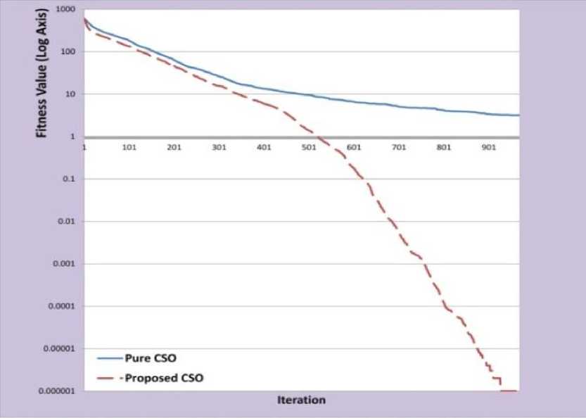
Fig. 2: Experimental Results of Rastrigin Function

As demonstrated in Figure 3 and Table 5, improved CSO in comparison with pure CSO, can find the better best solution in a same iteration.

Ackley’s function is a widely used multimodal test function [8]. It has the following definition

F(x) = -20. exp

(-0․2√ ¹ n∑x ^,

n

-exp( ¹ ∑cos(2πxi))-20

i=l

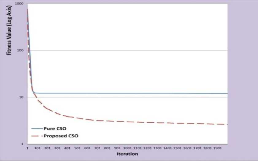
Fig. 3: Experimental Results of Griewank Function

Figure 4 shows that the proposed CSO can find the best solution of Ackley function in less iteration. As shown, proposed CSO can get the optimal solution in 1264th iteration. Meanwhile, the best solution of pure CSO is 0.004 in the 3500th iteration.

The axis parallel hyper-ellipsoid is similar to function of De Jong. It is also known as the weighted sphere

model. Function is continuous, convex and unimodal [8]. It has the following general definition

F(x) = ∑ i=l

i

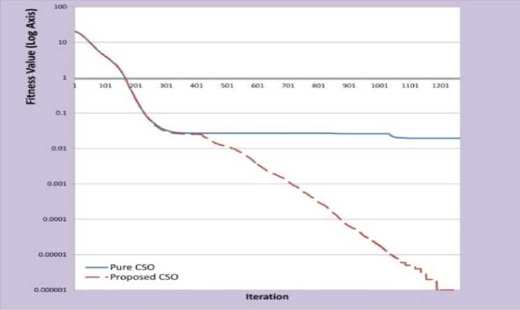
Fig. 4: Experimental Results of Ackley Function

As we shown in Figure 5 and Table 7, the optimal solution of axis parallel function is zero and both algorithms can find it. But the proposed CSO, in comparison with pure CSO can find it in less iteration.

The fifth function is Zakharov function. Zakharov equation is shown by (12).

n              / n \ 2

F(x) = ∑(x,)2 + (∑ 0․5ix, + i=l Vi=l /

n

+(∑ 0․5ix()4 i=l

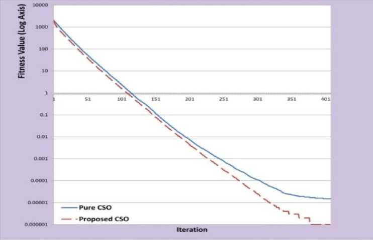
Fig. 5: Experimental Results of Axis Parallel Function

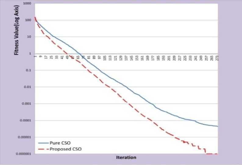
Fig. 6: Experimental Results of Zakharov Function

Figure 6 illustrates that the final solution of proposed CSO is better than pure CSO. It shows that proposed CSO can find the best answer in the 275th iteration which is 200 iterations less than pure CSO.

Trid10 function is the last benchmark for making a comparison between pure CSO and proposed CSO. It has no local minimum except the global one. Equation (13) shows the equation of Trid10 function.

10 10

F(x) = ∑(x, -1)2 - ∑x ,xi-1 (13) i=l i=2

Table 9 and Figure 7 show that the best solution of proposed algorithm is equal to -194.000593. In comparison with pure CSO, this value is closer to global minimum of function. (It is necessary to say that, due to many negative fitness values of Trid10 function, we added up the fitness values with number +194 in order to show the picture in log axis in Figure 7.

• V. Conclusion

In the optimization theory, many algorithms are proposed and some of them are based on swarm intelligence. These types of algorithms imitate the behavior of animals. Cat Swarm Optimization (CSO) is a new optimization algorithm for finding the best global solution of a function which imitates the behavior of cats and models into two modes. In comparison with Particle Swarm Optimization CSO can find the better global solution. But CSO is more complex than PSO and because of its complexity, sometimes takes a long time to find the best solution. So, by improving the pure CSO, we proposed a new algorithm namely ‘Adaptive Dynamic Cat Swarm Optimization’. First of all, we added an adaptive inertia weight to velocity update equation in order to facilitate the global and local search ability adaptively. Also we used an adaptive formula for updating the acceleration coefficient. Then, we used a new form of position update equation composing the novel position and velocity information. In new position equation, in addition to current information of position and velocity, we used the average information of two previous/next steps by applying a forgetting factor. Experimental results of six benchmarks indicated that the improved CSO in comparison with pure CSO has much better solution and achieves the best fitness value and converge in less iteration. Also by considering the process time, we found that our proposed algorithm runs faster than pure CSO.