A Novel Genetic-based Optimization for Transmission Constrained Generation Expansion Planning

Published Online December 2013 in MECS

Generation Expansion Planning (GEP) is the essential step in long-term planning problems, after properly forecasting the load for a specified future period. Generally, GEP is an optimization problem in which the objective is to decide the new generation plants in terms of what type and capacity they should be, where they should be installed and when to be invested, with the result that the cost function is minimized and various constraints are satisfied. GEP problem may be of a static type (for a specified stage, typically a year) or a dynamic type (for several stages in a specified period), concerning the stages under consideration for the planning horizon [1-3].

the 4-bus test system from Grainger & Stevenson for a planning horizon of one year and the IEEE-RTS 24-bus test system for a planning horizon of three years with growing complexity containing 16 and 288 decision variables, respectively, are used. EM is also applied to solve the TC-GEP problem for the Grainger & Stevenson 4-bus test system for a planning horizon of one year; the results of the GA are compared and validated against the EM. The results indicated that the GA is an effective alternative for the solution of the proposed TC-GEP problem.

• II.    Problem Formulation

• 2.1    Capital investment Costs

The capital investment costs along the planning horizon consists of generation investment costs and transmission enhancement costs as:

worst

I, = IG t + IT                                  (1)

At the following subsections, formulation of generation investment and transmission enhancement costs are discussed.

• A. Generation Capital Investment Costs

Generation investment costs in each year can be computed as:

In Formula (2), X is the number of type-p power plants placed on bus b ; CIGF denotes the fixed portion of the generation capital investment cost which is dependent on the number of power plants. CIGF can be determined as:

CIGF „ = CIGFT „ + CIGFL „ p , b                     p , b                    p , b

CIGFGC

+ CIGFP _h +

The terms in formula (3) refer to parts of CIGF which are concerning to technical, land, fuel piping costs and costs of interconnection into the main grid, respectively. Power plants composed of distributed units on network buses follow these rules:

Gas, steam and nuclear units placed on a bus where there is no other unit of the same type make up a new power plant.

Two gas units with a steam unit make up a combined-cycle power plant.

Maximum total capacity of each power plant is considered to be equal to 1,300MW.

In formula (2), Y denotes the number of type-k units placed on bus b ; CIGV is the part of generation capital investment costs which is variable with the number of units. CIGV can be calculated from formula k , b

among the buses. Increasing the number of power plants throughout distributing units among the network buses will increase the generation investment costs, whereas the transmission enhancement costs will be reduced by decreasing length-based overloads.

2.2 O&M Costs of Generation

M. = 222

f = 1 b = 1 k = 1

( HRG_t min x EG ^a" +

HRG max x EG¹" * ) x CFG _ k                i                       k , b

+ Com_t ” x EG‘ °‘ k , b             i

+ Com f “ x PG^k k , b

CIGV = CIGVT _h + CIGVL „ + CIGVP + k , b                       k , b                       k , b                      k , b

CIGVGC k , b

The terms in (4) refer to parts of CIGV which are concerning to technical, land, fuel piping costs and costs of interconnection into the main grid, respectively.

B. Transmission Enhancement Costs

As aforementioned, transmission enhancement requirements are considered proportional to the lengthbased overloads and are determined for a period of one year under the worst conditions (i.e., a period with the minimum reserve capacity). It is worthwhile to note that the transmission system model proposed in this paper is approximated and is not the only way to observe this point. The investment cost of transmission enhancement requirements is obtained from formula (5);

f ^{( i )}( x ) = p f^{( / - 1)}( x ) + qf ^{( i - 1)}( x - Ci)

ITT *   2 ( Z^ _x ( SL^ - SR ) _x CIT )           (5)

j = 1

Where CIT is the investment cost ($/MVA) of line j that requires to be enhanced; SL denotes power flow (MVA) through transmission line j under the worst conditions; _Z is set to 1 only if line j is overloaded, otherwise Z is set to zero; Two objective functions generation investment costs and transmission enhancement costs have conflicts in distributing units

Where P is the operation rate of generating unit and q =1-p indicates the unit’s Forced Outage Rate (FOR); c is generating capacity for unit in p.u ; energy generated by each unit is calculated by formula (8)

E_@ = Tp , J f ⁽ ' ^{- 1)} ( x)dx ^x i - 1

Where x i is equal to 2 C .

j = 1

• 2.3    Outage Cost

FOR of a generating unit represents the percentage of time the unit maybe unavailable due to unexpected outages. A generating unit maybe tripped at a rate given by it’s FOR. Some portion of the energy demand cannot be served owing to the FORs of the units and based on demand and available reserves. EENS is computed from formula (9) and cannot be equal to 0; rather, it should be minimized as a cost term called outage cost, specified by formula (10):

x max + C t

EENS = T J f ⁽ n ) ( x )dx

C t

O t =

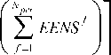
+ C x l У EENS^f

V f = 1

Where EENS^f,t denotes EENS (MWH) in period f , and year t of the study period; c t is the total capacity of all of the active generating units during the time interval; a , b and c are constants; and ELDC of the PPS is also used to calculate EENS and loss of load probability(LOLP) used in the constraint objective[12]. LOLP can be calculated from formula (11).

Where the first and second terms refer to presentworth values of capital investment costs and O&M costs, respectively. In addition, the third and fourth terms represent the present-worth value of outage costs and power active loss costs, respectively. S is the salvage value of the investment costs, which is deducted from the capital investment costs. In order to calculate the present-worth value of the cost components of formula (13), it is supposed that the full capital investment for a plant or a transmission equipment added by the expansion plan are made at the beginning of the year in which it goes into the service. As a matter of fact, the present-worth factors are specified with this assumption.

• 2.6    Constraints of the Proposed Method

Two types of constraints are considered in the proposed TC-GEP problem: fuel constraints and technical constraints.

A. Fuel Constraints

As can be seen from formula (14), each fuel supply center is able to supply a maximum amount of generation capacity.

NU

FUV e + У ( FUV _ x EG^to o x U_ ) <  FUV max m , t                           m , i             i , t          i , t                    m , t

i=1                                                    (14)

LOLP = f ⁽ n ) ( C )

V m = 1,..., N,t t = 1,..., T

• 2.4    Transmission Losses Costs

The costs of active power losses can be calculated as:

Lt

NL

CLT x £ ( RL j x ( IL j ) )

Where IL j denotes the current of line j which is calculated by solving the AC load flow for the system involving candidate units. As aforementioned, in this model, it is assumed that the network load is uniformly increased between the network load buses according to the forecasting load for each year.

• 2.5    Objective Function of the Proposed Method

As aforementioned, the discounted value of the total generating costs is considered as the objective function, which is represented by formula (13):

T

Min C = У [ I_t + M_t + O_t + L - S ]           (13)

t = 1

B. Technical Constraints

There are uncertainties that may cause generation units to trip unexpectedly at any time. Consequently generation capacity should be adequate in satisfying the load requirements. The following two constraints, then, should be taken into account:

(1 + a, ) D,  > ?(k,  )>(1 + b ) D, t        t,c                  t,c                      t        t,c

V t = 1,..., T

LOLP < LOLP t           max

V t = 1,..., T

Where c is the critical period. It denots the period of the year in which the difference between the relevant available generating capacity and the peak demand has the smallest value. Formula (15) clearly implies that the installed capacity in the critical period must lie between the given maximum and minimum reserve margins— a_t and b_t , respectively—above the peak demand ( D_t,c ) during the critical period of the year.

In the proposed TC-GEP problem, the reliability of the system is computed in terms of the LOLP index for each period of the year, as in formula (16). The LOLP of each period is specified as the average annual LOLP, where the sum of the LOLP of the periods is divided by the total number of periods.

• III.    Solution Methodology

• 3.1    Applying a GA to the Proposed Method

As previously mentioned, the purpose of this problem was to find the optimum number, type and location of the candidate generating units. The objectives are described in Section 2.In the following section, a GA is employed to the proposed method.

In nature, each species must adapt itself for the maximum likelihood of survival in a challenging environment. Species with improved characteristics tend to survive overtime. In fact, species with higher fitness levels survive longer. This type of phenomenon, which occurs in nature, is the basis for the evolutionarybased GA [1,13-15].To solve a TC-GEP problem using a GA problem, variables are combined and represented as mixed integer coding in each chromosome. The data structure of the chromosome can be depicted, as shown in Figure 1. As can be seen from this figure, each three genes of the chromosome refer to the number of type-k plants on bus b, in year t of the study period. In the proposed GA, candidate solutions of the initial population are randomly selected between all solutions to satisfy the constraints in formula (15), and new solutions are obtained through the GA’s operators (selection, crossover, and mutation) which are checked to sustain feasibility.

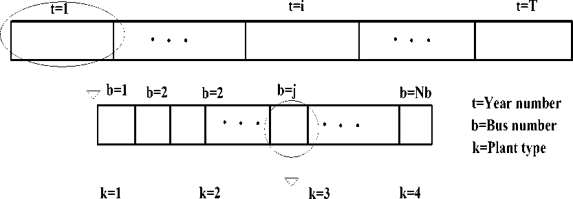
Fig. 1: Data structure of each chromosome of GA

• IV.    Sinulation

• 4.1    Case Study 1

У

U318

As can be seen from this figure, there is only one fixed nuclear unit of 318MW nominal capacity, and 8% FOR, which is placed on bus 4; total network load is 500MW. For this case study, the TC-GEP problem is solved for a planning horizon of one year. First, a GA is used as the optimization tool, then the Enumeration Method (EM) is used to solve the problem for all feasible chromosomes, satisfying formula (15).

As can be seen, the candidate plants are distributed on buses 1 and 3. Capital investment costs related to various factors (technical, land, fuel piping and interconnection to the main grid) of the candidate units for the expansion plan proposed for Case study 1 are presented in Table 2. As can be seen from this table, two steam and natural-gas power plants are developed by distributing candidate units between buses 1 and 3. Also, the expected energy not served, overload, active power losses and the discounted value of all of the cost terms of the objective function for the proposed expansion plan for case study 1 are presented in Table 3. Total objective function for case study 1 is equal to $1,059,931,580. The GA converges at the 4th iteration.

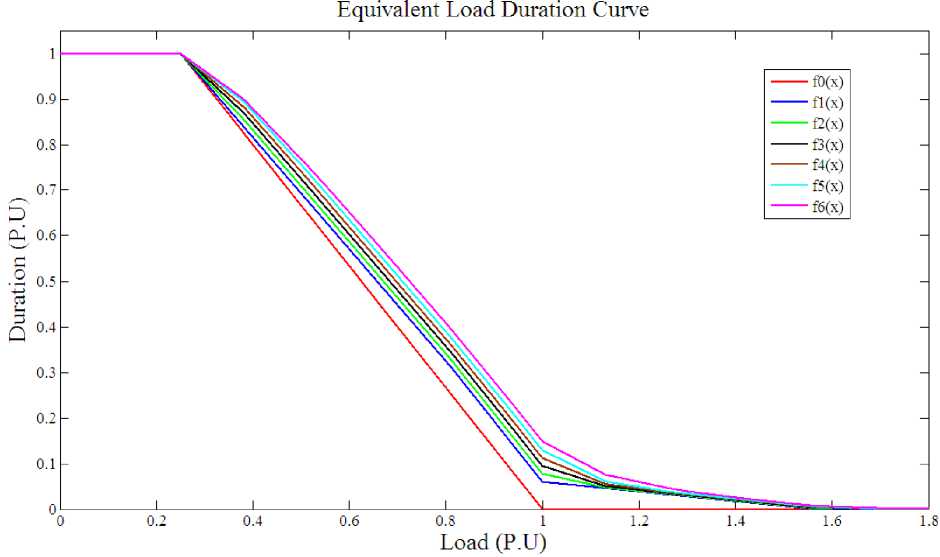
Fig. 3: ELDC for case study 1

Unit number	Unit type	Bus Number	Unit Type	Total Generated Energy (GWH)	Generated Energy in base Capacity (GWH)	Fuel costs (K$)	Non-fuel O&M costs (K$)	O&M cost involving fuel costs (K$)
1	Fixed	4	U318	567.95	181.33	7951.35	737.63	8688.99
2	Candidate	3	F-CC	79.96	40.28	1193.65	246.41	1440.07
3	Candidate	3	F-CC	58.46	36.2
4	Candidate	1	FOIL	35.96	32.11	6925.83	1657.07	8582.9
5	Candidate	1	FOIL	16.4	4.1
6	Candidate	1	FOIL	16.24	10.43
7	Candidate	1	FOIL	4.04	1.01
Total	-	-	-	779.01	305.46	16070.83	2641.11	18711.96

Table 2: Capital investment costs for Case study 1

Terms/ Power Plant Number	Power Plant type	Bus Number	Unit Number	Technical costs (K$)		Land costs (K$)		Fuel piping costs (K$)		Costs of interconnection to the main grid (K$)		Fixed costs (K$)	Investment Costs (K$)
				Depreciable	Nondepreciable	Depreciable	Nondepreciable	Depreciable	Nondepreciable	Depreciable	Non-depre-ciable
1	NGAS	3	2	893.6	0	80	0	135	0	82	0	150781.82	153163.02
			3	893.6	0	80	0	135	0	82	0
2	STEAM	1	4	2960.4	148	310	155	15.27	7.63	35	0	103818.18	118343.38
			5	2960.4	148	310	155	15.27	7.63	35	0
			6	2960.4	148	310	155	15.27	7.63	35	0
			7	2960.4	148	310	155	15.27	7.63	35	0
Total				13628.8	592	1400	620	331.08	30.52	304	0	254600	271506.3

Table 3: Value of all cost terms of objective function for the expansion plan proposed by GA for Case studies 1 and 2

Terms/ Expansion plan proposed by GA	Year number	Expected energy not served (GWH)	Overload (MVA)	Active power losses (MW)	O&M cost (K$)	Capital investment cost (K$)	Salvage value of capital investment cost (K$)	Outage cost (K$)	Transmission enhancement cost (K$)	Active power losses cost (K$)	Objective function (K$)
Case study1	1	3.217	74.943	5.81317	69561.669	1621617.09	1403320.0396	647100.98	123460.24	1511.63	1059931.58
Case study 2	1	0.318438	13.472128	54.7463	288180.33	860016.872	604981.32	43801.159	14618.101	14235.99	615871.127
	2	0.096564	411.6279	131.461	348381.41	1044793.611	801774.432	11660.672	415628.523	31077.014	1049766.803
	3	0.08349	682.3472	258.482	334248.126	601305.334	531660.627	9147.969	827778.368	55549.241	1296368.412
	Total	0.4984	1107.44	444.689	970809.871	2506115.818	1938416.387	64609.801	1258024.993	100862.246	2962006.343

• 4.2    Case Study 2

An IEEE-RTS 24-bus test system is selected as the second case study to which the TC-GEP problem is applied for a planning horizon of three years with growing complexity [17-18]. Figure 4 shows this test system. As can be seen from this figure, there are 32 fixed units of 3,405MW total nominal generating capacity. Total network load is 2,850MW, and it is assumed that the network load would uniformly increased between the network load buses.

The proposed GA that is validated for case study 1 and compared with the EM is also employed to solve the TC-GEP problem for this case study. The expansion plan suggested by the GA for case study 2 is shown in Table 4. As can be seen, 8 power plants consisting of 18 units each are distributed between buses 7, 11, 12 and 17.

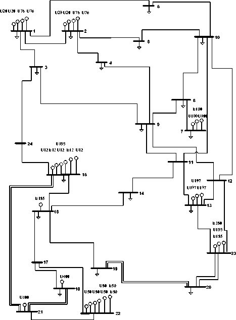
Fig. 4: Case study 2: IEEE-RTS 24-bus test system

Table 4: Specification of expansion plan proposed by GA for Case study 2

Year number	Power plant number	Power plant type	Power plant capacity	Bus number	Unit number	Unit type
1	1	STEAM	280	11	1	FCOA
	2	NGAS	174	11	2	F-CC
	3	CCYC	628	12	3	F-CC
					4	F-CC
					5	FCOA
2	4	CCYC	454	7	6	F-CC
					7	FOIL
	2	NGAS	348	11	8	F-CC
	3	CCYC	983	12	9	FOIL
					10	FCOA
	5	NGAS	174	17	11	F-CC
	6	NUCL	400	17	12	NUCL
3	4	CCYC	529	7	13	FOIL
	7	STEAM	355	7	14	FOIL
					15	FCOA
	1	STEAM	355	11	16	FOIL
	3	CCYC	1263	12	17	FCOA
	8	STEAM	35	17	18	FOIL

Terms/Year number	Fuel costs (K$)	Non-fuel O&M costs (K$)	O&M cost involving fuel costs (K$)	Technical costs (K$)		Land costs (K$)		Fuel piping costs (K$)		Costs of interconnection to the main grid (K$)		Fixed costs (K$)	Investment costs (K$)
				Depreciable	Nondepreciable	Depreciable	Nondepreciable	Depreciable	Nondepreciable	Depreciable	Nondepreciable
1	285685.879	46784.809	332470.688	240689.76	16119.6	24948	14870.8	20745.2	9872.8	7364.4	0	611408	946018.56
2	381485.183	60784.4587	442269.642	539880.75	9971.9	34936	9318.95	16581.725	5179.725	6856.9	0	682000	1304725.95
3	390233.168	76499.263	466732.432	280092.5	20461.9	23010	17178.15	12089.125	10003.725	4002	0	433500	800337.4
Total	1057404.23	184068.53	1241472.762	1060663.01	46553.4	82894	41367.9	49416.05	25056.25	18223.3	0	1726908	3051081.91
				1107216.41		124261.9		74472.3		18223.3

• V.    Conclusions

Acknowledgments