A Novel Hybrid Model for Brain Tumor Analysis Using Dual Attention AtroDense U-Net and Auction Optimized LSTM Network

Published Online on February 8, 2026 by MECS Press

The human brain stands as the most complex and highly organized structure within the human body, essential for various cognitive and physical functions [1]. However, its complexity also makes it susceptible to abnormalities, such as tumors. Brain tumors form when healthy brain cells grow uncontrollably, disrupting normal function. A healthy brain consists of three primary tissues: white matter, grey matter and cerebrospinal fluid. Accurately identifying and segmenting brain tumors within these tissues is critical for early diagnosis and effective treatment planning [2]. Among the available imaging techniques, magnetic resonance imaging (MRI) is the preferred method because of its non-invasive nature and superior tissue contrast, without the use of radiation [3]. MRI types, such as T1-weighted, contrast-enhanced T1-weighted, T2-weighted and FLAIR, provide valuable data for analyzing tumor subregions [4,5].

Segmentation of tumors from MRI aims to pinpoint their location and extent. This process plays an important role in medical evaluation, enabling appropriate intervention and better outcomes. Though traditional manual segmentation methods are widely used, they are labor-intensive, time-consuming and susceptible to errors, particularly due to the complexity of brain anatomy and the variability in MRI images. [6,7]. Furthermore, noise, artifacts and low resolution images are additional factors that hinder efficient tumor detection and classification. These challenges make it essential to design automatic tools for effective and reliable tumor recognition These challenges necessitate the development of automated tools for reliable and efficient tumor diagnosis. Artificial intelligence (AI) has become a promising tool in medical image processing by utilizing machine learning (ML) and deep learning (DL) algorithms for segmentation and classification tasks [8,9]. Among these, deep learning-based approaches have shown superior accuracy and consistency in extracting and analyzing tumor features. These models can effectively differentiate between regular and pathological brain tissues, overcoming the limitations of traditional methods [10,11].

Tumors can be classified as benign or malignant tumors. The secondary tumor originates from other organs and spreads to brain where it grows into tumor [12]. Accurate classification of these tumor types is crucial for determining the necessary treatment plans and automated diagnostic tools must reliably identify tumor regions, accounting for their diverse size, irregular borders and location. This is particularly challenging given the existence of noise and artifacts in MRI images. Moreover, low-resolution images and anatomical complexities pose additional hurdles in segmentation and classification [13].

Recent advancements in medical image processing in the last few years have introduced sophisticated deep learning-based models capable of addressing these challenges. These methods focus on segmenting tumor regions, classifying tumor types and facilitating early diagnosis to improve survival rates. Research shows that deep learning algorithms can produce better and reliable results. This work develops a new method for tumor segmentation and classification, using AI techniques to overcome current challenges.

2.    Related Works

Various approaches for classifying and segmenting brain tumors were studied in this work. The following are the more recent and efficient ones:

Saeed Iqbal et al. [14] proposed a Fusion Net framework using ResNet and employed various preprocessing techniques and integrated radiomic features to improve the detection of diseased patches, achieving an F1 score of 96.72, precision of 97.7, specificity of 96.31 and accuracy of 97.5 from BraTS dataset.

Atika Akter et al. [15] proposed an automated tumor detection and classification model for MRI images. It was developed by integrating a CNN-based classification model and a U-Net-based segmentation model. The model attained remarkable results, with classification accuracies of 98.7% and 98.8% when using the segmentation approach, surpassing pre-trained models in performance. The framework also demonstrated a high accuracy of 97.7% on individual datasets, showcasing its robustness and applicability for clinical use. However, the inclusion of more diverse and real-world MRI data would additionally improve generalizability and effectiveness.

Abdullah A. Asiri et al. [16] introduced a novel two-part model, first module utilizes wiener filter, neural networks and ICA to remove artifacts and improve low contrast. The second module employs Support Vector Machines (SVM) for segmentation and classification. This approach, was tested on various tumor and got an accuracy of 98.9%, sensitivity of 99.1%, specificity of 99.1% and a Dice score of 98.1%. Future advancements aim to enhance the system's robustness by adopting standardized multi-classifier techniques.

Nechirvan Asaad Zebari et al. [17] introduced a fusion approach that mixes VGG16, ResNet50 and Convolutional Deep Belief Networks (CDBN) to improve tumor classification accuracy. By leveraging data augmentation to increase the training dataset and utilizing Softmax as classifier, the fusion model achieved an accuracy of 98.98%, surpassing individual networks by 5.33% (VGG16), 1.78% (ResNet50) and 3.3% (CDBN). Future directions include exploring transfer learning techniques and larger datasets to enhance model stability, reduce reliance on augmentation and further support automated tumor diagnosis in clinical settings.

Asma Alshuhail et al. [18] presented a DL based method using convolutional neural networks (CNNs) with a sequential architecture for classification. The model got a diagnostic accuracy of 98%, with precision, recall and F1-scores between 97% and 98% and a ROC-AUC score between 99% and 100% for each tumor classes.

Sarfaraz Natha et al. [19] addressed the urgent need for early tumor detection by using a Stack Ensemble Transfer Learning model. This method combines two pre-trained networks, AlexNet and VGG19, to different tumors types. The SETL_BMRI model achieved an accuracy of 98.70%, along with precision, recall and F1-scores of 98.75%, 98.6% and 98.75%, respectively. However, challenges related to dataset size and class imbalance were encountered.

Samar M Alqhtani et al. [20] introduced a multiple stages model including preprocessing with Contrast Limited Adaptive Histogram Equalization and diffusion filtering to improve MRI image coherence, followed by tumor region segmentation using the Fuzzy C-Means (FCM) and SVM classifier. The method demonstrated exceptional performance, achieving sensitivity, specificity, accuracy and a Dice score of 0.977, 0.979, 0.982, 0.961 respectively. Despite these promising results, the approach faced several limitations, such as limited generalization to diverse datasets, dependence on image quality, sensitivity to parameter settings and the lack of clinical validation.

Khan et al. [21] proposed a DL approach for tumor classification using MRI. In the pre-processing stage, image intensities were utilized to address noise in the images, with normalization achieved by calculating the average values across different image slices with varying intensities. The region of interest (ROI) from MRI scans was then segmented using the k-means clustering. Finally, classification was performed using the VGG19 network model, with the BraTS2015 dataset employed for evaluation.

Aboelenein et al. [22] developed a brain tumor segmentation model based on a 2D HTTU-Net architecture. The BraTS2018 dataset was utilized for the quantitative assessment of the proposed model. To address the class imbalance issue, a hybrid loss function was developed by uniting the focused loss and dice loss functions. The primary limitation of the proposed method was its lengthy training phase.

Díaz-Pernas et al. [23] introduced an automatic segmentation and classification method using a Deep Convolutional Neural Network (DCNN). The multiscale CNN employed three pathways for tumor segmentation and classification into various types. It achieved an accuracy of 97.3%, with data augmentation applied to prevent overfitting and enlarge the dataset.

Nayak et al. [24] proposed a dense EfficientNet, a variant of CNN, for tumor classification, achieving an accuracy of 98.78%. To improve the results, min-max normalization and data augmentation were applied. However, the method's limitation was its high computational time.

Rajeev et al. [25] introduced a hybrid DL method to classify brain tumors from the Kaggle dataset. Features extraction and feature selection were done using an improved gabor wavelet transform and hybrid BWARD algorithm. A combination of Elman RNN and BiLSTM was used to classify the tumor into different types. The suggested model outperformed existing models and 98.4% accuracy was obtained; however, multimodal MRI images were not used.

Khan et al. [26] proposed a 3D Hybrid Attention-Based Residual U-Net (HA-RUnet) for brain tumor segmentation in MRI volumes. The model integrates residual blocks with attention and squeeze–excitation modules to enhance multi-level feature learning while maintaining low computational complexity. Using the BraTS-2020 dataset, the method achieved Dice scores of 0.867, 0.813, and 0.787 for whole tumor, tumor core, and enhancing tumor, respectively, outperforming standard ResUNet models.

Lin and Lin [27] proposed a brain tumor segmentation framework that integrates EfficientNetV2 as the encoder within a U-Net architecture to enhance feature extraction efficiency and segmentation accuracy. The approach leverages U-Net skip connections to retain multi-scale contextual information while EfficientNetV2 improves representation learning. The method was evaluated on glioma MRI data and achieved a Dice similarity coefficient of 0.9133 with an accuracy of 0.9977.

Li et al. [28] developed a multi-scale deep residual U-Net (mResU-Net) for automated brain tumor segmentation in MRI. The model adopts residual learning to mitigate gradient vanishing and employs multi-scale convolution kernels and channel-attention modules to enhance feature representation across varying tumor sizes. Skip connections are retained to reduce the semantic gap between encoder and decoder. Evaluation on the BraTS-2021 dataset yielded Dice scores of 0.9289, 0.9277, and 0.8965 for tumor core, whole tumor, and enhancing tumor, respectively.

Each technique has the drawback of requiring large datasets for model training to yield useful results. Additionally, the model's lengthy training period prevents some research assets from being used for quick analysis. Current systems employ various methods, such as model-based, hybrid-based and threshold-based segmentation, all of which have a number of downsides, including longer processing times and higher error rates. This study intends to effectively implement deep learning-based techniques to reduce these drawbacks and improve classification accuracy.

3.    Materials and Methods

Brain tumor detection is critical for reducing mortality rates associated with late diagnosis. Early and accurate identification of tumor regions in MRI images is essential for effective treatment planning. DL based models have offered significant improvements in classification accuracy compared to traditional approaches. This study proposes a novel DL-based framework to automatically and reliably segment and classify tumor regions. The method involves five key stages: pre-processing, segmentation, feature extraction, feature selection and classification. The stages of the proposed methodology are shown in Fig. 1.

• 3.1.    Dataset Description

  The Brain Tumor Segmentation Challenge (BraTS) datasets [29-31] are gold standard dataset used for Brain tumor segmentation and classification. The BraTS 2019 and 2020 datasets provide multi-modal MRI scans of brain tumors, including T1-weighted (T1), T1-weighted contrast-enhanced (T1ce), T2-weighted (T2) and T2 Fluid Attenuated Inversion Recovery (T2-FLAIR). For each MRI scan, expert radiologists have manually annotated the tumor region which serve as the gold standard for analysing the segmentation models. The BraTS2019 dataset includes a total of 1,675 MRI images, with 1,295 images of HGG and 380 images of LGG. In contrast, the BraTS2020 dataset contains 1,435 HGG images and 281 LGG images. For testing, 393 images from BraTS2020 were used, while 919 images were used for training. Similarly, in the BraTS2019 dataset, 492 and 1,435 images were used for testing and training respectively. These experiments were conducted using an internal train–test split rather than the official BraTS validation server. Patient-level separation was not explicitly enforced in the original implementation.

3.2. Pre-processing

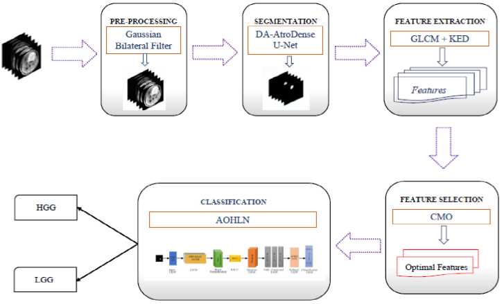
Fig.1. Block diagram of the proposed approach

MRI scans often include distortions and artifacts caused by environmental factors and imaging technology. In order to prepare MR images for further processing, non-brain sections of the image are removed, non-uniform properties are corrected and MR images are brought into a single common spatial and intensity space. In the preprocessing step a Gaussian bilateral filter is used for noise removal. This filter smooths the image while preserving important edge details by weighting pixel values based on spatial proximity and intensity similarity. It assures a clearer image for subsequent processing steps. In this work, the bilateral filter is used only as a light stabilization step to suppress random background noise while retaining structural boundaries as defined in (1) –(5). It is acknowledged that modern CNN models are capable of internal denoising; therefore, the bilateral filter is not intended to replace learned feature extraction, but to provide a cleaner and more consistent input image prior to segmentation.

I’(p) = У * G_s)(p) = S_RIW)G_s ⁽ p - q) dq

G_s ⁽ p-q) = exp (- ^т- т- )

20s

j,, , _ [gdq)Gs(:p-c№r№

^P       !_RG_s(p-q}G r (l(p}-I(q})dq

G_r(l(p) - I(q)) = exp (- (^^

W(p) = J_R G_s ⁽ p - q)G r (/ ⁽ p) - I ⁽ q) dq

where I (p) is Intensity of the pixel at position p in input MRI, Г (p) is Output (filtered) intensity at position p,q: is neighboring pixel location relative to p, G_s(p — q): Spatial Gaussian kernel, G_r(l(p') — I(q)): Range Gaussian kernel, a : Spatial standard deviation, determines the extent of spatial smoothing and a _r is the Range standard deviation and W(p) is the Normalization factor ensuring proper weighting as given in (5). The overall objective is to retain clinically meaningful edge information while reducing random noise, without introducing excessive smoothing that may degrade fine tumor texture.

• 3.3.    Segmentation

The Dual Attention AtroDense U-Net (DA-AtroDense U-Net) is an advanced architecture designed for robust and accurate tumor segmentation. The term AtroDense denotes the integration of atrous (dilated) convolutional layers with densely connected feature blocks within the U-Net framework. The network is built on the conventional U-Net encoder–decoder structure for pixel-level image segmentation, while incorporating three key enhancements: dual attention mechanisms, atrous convolutional layers and dense blocks with lightweight reductions. Atrous convolutions enlarge the receptive field without reducing resolution, whereas dense connectivity encourages feature reuse and alleviates vanishing-gradient effects. By combining these components, the DA-AtroDense U-Net is capable of capturing multi-scale contextual information, preserving spatial detail and improving learning efficiency, thereby providing a highly effective solution for medical image segmentation. Challenges such as boundary ambiguity, spatial information loss and computational overhead can be reduced through this architectural design.

In the proposed model, dense blocks are embedded within both encoder and decoder paths to ensure that feature maps from preceding layers are concatenated and re-used throughout the network, leading to richer representation learning. Dual-attention modules are applied to the encoder feature maps before transfer through the skip connections. The position-attention component enhances spatially discriminative tumor-region responses, while the channel-attention component amplifies the most informative feature channels. The attention-refined feature maps are then concatenated with the decoder activations, enabling more accurate tumor localisation while preserving fine structural boundaries.

U-Net is most often used architectural models for biological semantic picture segmentation. However, U-Net faces challenges such as the "gradient vanishing problem", where gradients in initial layers diminish during training and the loss of local information and spatial details due to convolution and non-linearity operations. To address these issues, in this work, a standard U-Net is enhanced with Atrous Convolutional Layers, Dual Attention Mechanisms (position attention module (PAM) and channel attention module (CAM).

The encoder extracts multi-scale features through successive Atrous Convolutions integrated with dense blocks. Each encoding stage downsamples the input feature maps using atrous convolution with stride and feeds them into dense blocks. Atrous convolution widens the filter's view without adding computational cost or losing spatial detail. It is defined in (6) as:

(F *_r W)(p) = Y k F(p + r - к) ■W(k')                                 (6)

where F represents the input feature map, W the convolution kernel, r is the dilation rate and p is the current pixel position. The decoder reconstructs spatially detailed feature maps from the encoded features using an Atrous Decoder. The atrous decoder leverages the indices of maximum activations from the encoder’s pooling layers to restore the spatial details lost during down-sampling. The decoder's upsampling operation ensures that spatial information is restored while integrating multi-scale contextual data. It uses the saved pooling indices and performs the operation defined as (7):

U_d(x,y) = Max({F_e(i,j) | i,j E indices(x,y)})                                (7)

where F_e is the encoder feature map and (x, y) are the spatial coordinates.

Dense blocks are the building units of both encoder and decoder. Unlike conventional convolutional layers, dense blocks concatenate feature maps from all preceding layers, encouraging feature reuse and alleviating the vanishing gradient problem. For a dense block with L+1 layers, the output of the ℓ+1th layer is defined in (8) as:

X i+i = H^X o^i,...^])                                    (8)

Here, H f represents a composite function (convolution, batch normalization and ReLU) and [x₀,x 1 , .,x ^\ denotes the concatenated inputs from all previous layers. To reduce computational overhead, traditional convolutions is replaced with lightweight layers having 1×1 convolutions which reduce the number of input channels and 3×3 convolutions perform feature extraction.

The dual attention mechanism refines the feature maps by focusing on relevant spatial (PAM) and channel-wise (CAM) information. PAM enhances spatial feature extraction by learning pixel-wise relationships. An attention weight map is calculated and then used to scale the encoder's feature map as in (9) and (10).

F pam = aQF                                  (9)

a = a(^(F _enCo_der ) + ф(F decoder ))                                      (10)

where a is the attention weight map, ф and ф are convolutional transformations, a is sigmoid activation function and element-wise multiplication is represented using О ■

CAM emphasizes channel-wise dependencies, learning inter-channel relationships. It uses global average pooling (GAP) and fully connected layers as defined in (11) and (12).

s_c = a(W 2 ■ ReLU(W i ■ Z)) ^^^Mj)

where Z_c is the GAP vector, W 1 and W 2 are weight matrices of fully connected layers and a is the sigmoid activation function.

The decoder reconstructs the feature maps to the original image size using atrous upsampling. It restores spatial dimensions using indices saved during pooling in the encoder as defined in (13).

^ decoder    ^UnpOOl(f encoder indices )

The final segmentation map is generated using a 1×1 convolution applied to the output of the last dense block as expressed in (14).

P(x) = Softmax(W * F + b)

P(x) is the probability map, W and b are learnable weights and biases and * denotes convolution.

Fig.2 shows the atrous encoder block and Fig.3 shows the architecture of the DA-AtroDense U-Net model.

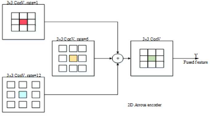
Fig.2. 2D Atrous encoder block diagram

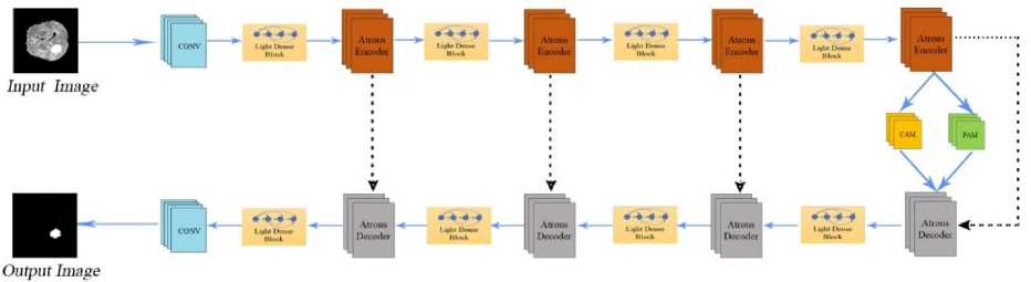
Fig.3. Architecture of dual attention Atrodense U-Net

In the proposed DA-AtroDense U-Net, the encoder path consists of a sequence of atrous convolutional blocks interleaved with lightweight dense blocks. Each lightweight dense block concatenates the feature maps from all preceding layers within the block, thereby encouraging feature reuse and improving gradient propagation while keeping computational overhead low. The atrous encoder blocks enlarge the receptive field without down-sampling, allowing the network to capture long-range contextual information that is important for tumor boundary perception.

The corresponding decoder path mirrors the encoder structure using atrous decoder blocks and lightweight dense units to progressively reconstruct high-resolution feature maps. Skip connections transfer encoder features directly to the decoder to recover lost spatial detail. Prior to the final decoder stage, dual-attention mechanisms are applied. The channel-attention module (CAM) emphasises the most informative feature channels, while the position-attention module (PAM) enhances spatially discriminative tumor-region responses. The attention-refined feature maps are then fused with the decoder output, ensuring that the network remains focused on clinically-relevant tumor regions while retaining fine anatomical details.

• 3.4.    Feature Extraction

After segmenting the tumor regions using the DA-AtroDense U-Net, feature extraction is performed to derive meaningful characteristics of the segmented regions for further classification or analysis. In this work, the classification stage is intentionally designed around handcrafted texture features, as tumor heterogeneity is often reflected in local intensity and texture variations that are clinically relevant. While the U-Net is primarily optimised for accurate boundary localisation, the features learned in its latent space are not explicitly constrained to preserve radiomic texture indications. Therefore, the feature extraction process combines the Kirsch Edge Detector (KED) for edge-based structural information and the Gray Level Co-occurrence Matrix (GLCM) to quantify texture descriptors such as contrast, entropy, energy and homogeneity. These handcrafted features are not fused with the deep-learning feature maps. This hybrid design allows the framework to retain the advantage of deep-learning-based segmentation while incorporating explicit and interpretable tumor texture characteristics for classification.

The Kirsch Edge Detector is a non-linear edge detection algorithm designed to detect edges in multiple directions, capturing abrupt intensity changes, which are crucial for recognizing tumor boundaries.

KED uses a set of convolution kernels that identifies edges by calculating the maximum gradient in eight compass directions (N, NE, E, SE, S, SW, W, NW). The Kirsch filter applies a kernel matrix to a pixel and its neighbors to compute directional gradients. For a pixel intensity I(x,y) the gradient G_k in the k-th direction is given in (15) as:

G_k ^^-iX^-iKkttj) ■ I⁽x + i,y + j)                             (15)

where K_k(i,j) is the к — th Kirsch kernel, I(x + i,y + j) represents the pixel intensity in the neighborhood. The final edge magnitude at each pixel is: G (x, y) = max G_k where k ranges over the eight compass directions.

k

GLCM is used to analyze texture by considering the spatial relationship of pixels. It determines the frequency of pixel intensity pair’s occurrences at a specified offset and direction.

Given an image I, the GLCM P(i,j) is defined in (16) as:

p(i,j,d,e) = #{(x1,y1),(x2,y2) e I:I(x1,y1) = i,I(x2,y2) =j}(16)

From the co-occurrence matrix, statistical features like contrast, correlation, energy and homogeneity are derived. These features characterize the texture patterns of the tumor region, such as smoothness, granularity, or randomness as defined in (17)-(20).

Contrast = Xi,jP(i,j) ■ (i — j)2(17)

Homogeneity = £ц Pj-.

, ¹⁺li-j|

Entropy = — T^ P(i,j) ■ log(P(i, j))(20)

The edge-detected image from KED highlights regions with sharp intensity transitions and then GLCM is applied to these edge-enhanced regions to extract texture features, focusing on the area’s most likely to contain meaningful details. The extracted features improve the discriminatory power of ML or DL models used for tumor classification.

• 3.5.    Feature Selection

A vital role in reducing redundancy and selecting the most relevant features for classification tasks is played by feature selection. In this work, the Cat-and-Mouse Optimization (CMO) algorithm is employed to select a compact subset of texture features by reducing redundancy and correlation among the extracted GLCM descriptors. This strategy improves the relevance of the retained features and stabilises classification performance in a high-dimensional feature space where exhaustive search is infeasible. The use of CMO is intended purely as a performance-supporting mechanism rather than as an algorithmic novelty and conventional selection strategies remain valid alternatives. The CMO is an optimization algorithm based on natural interaction between cats and mice. Mice attempt to flee to safe havens, while cats play the role of pursuers trying to catch them. The algorithm simulates this behavior to explore and exploit the search space, eventually selecting the optimal subset of features.

The possible solutions are represented by the population matrix as shown in (21), where each solution is associated with a collection of features. A combined population of N agents is represented as a matrix. The total population is divided equally into N_c cats and N_M mice (N=N_c +N_M).

	\ p1,1    ■	P 1,n	■    P1,D '
p =	P il   -	pi,n    "	P i,D
	-PN1	"  Pn, n	"    pN,D -

where p_i j - value of the j-th problem variable for the i-th agent, N - number of search agents and D - number of problem variables or features. Each agent's position (feature subset) is evaluated using an objective function f(p_i) which assesses the quality of the selected features based on feature relevance and redundancy is given in (22).

f(P t ) = a ■ (1- Corr(X_p.)) + P ■ Variance(Х_р^

where p_i is the feature subset selected by the i-th agent, Corr(Xpi) is the correlation coefficient matrix of the selected features, Variance (Xpi) is the variance of the selected features and α, β are the weighting factors balancing correlation reduction and feature variance. After evaluating all agents, the population is sorted in ascending order based on their objective function values. Agents with lower f(p_i) values are considered better solutions, as they indicate lower feature correlation and higher variance.

In the first stage the cats update their positions by moving toward the mice and it is defined in (23) as:

„ new                           i   f(P e )

^pi,k     ^pj,k ^{+ r} ■ ^(pe,k    ^pj,k ) ■ f(pj)

where, pⁿ_k - updated position of the jth cat in the kth dimension, P i _k - current position of the jth cat in the kth dimension, p_ek -position of the eth mouse in the kth dimension, f(p_e) is the fitness of the eth mouse and f(pi') is the fitness of the jth cat and r -random number in the range [0, 1].

In the next stage mice update their positions to move toward safe havens s_i which is generated randomly within the search space as defined in (24) and (25).

s i,k = randU k , U k )

P ik = P ik + ^r ■ ^(si,k ^- P ik )

where, s_{i k} denotes the safe haven position for the ith mouse and p i ^e _k is the updated position of the i-th mouse.

After updating positions, the objective function values are recalculated for each mouse. The fitness function evaluates the value of the selected features based on correlation and classification accuracy. The correlation between two features x_k and x_t is calculated in (26) as:

Corr(x_k, x i ) =                                                             (26)

V Z (x k -x k ) ²VX^(x l ^-x l ⁾²

The fitness function aims to minimize feature correlation and maximize feature variance, ensuring that selected features are both diverse and informative as defined in (27).

f(Pi) = a ■ (^X k-^k+i Corr(X k ,x) - P ■ 1^=1 Var(X k )                   (27)

where n represent the number of selected features, Corr(x_k, X [ ) is the correlation between features к and I, Var(x ^ represents the variance of feature к.

The CMO algorithm iteratively update the positions of the cats and mice, evaluating the fitness of each solution. By minimizing correlations between features, the CMO ensures that only unique and relevant features are retained. The dual-stage process (cats pursuing and mice escaping) ensures a balanced exploration and exploitation of the search space.

• 3.6.    Classification

An innovative deep learning architecture called the Auction-Optimized Hybrid LSTM Network (AOHLN) was created to accurately categorize brain tumors from MRI-derived radiomic features. It brings together the benefits of Long Short-Term Memory (LSTM) networks and the Auction-Based Optimization Algorithm (ABOA) to accomplish high accuracy and robustness. The term “auction-optimized” denotes that the LSTM weights are then fine-tuned using an Auction-Based Optimization Algorithm (ABOA), which functions as a meta-heuristic weight refinement strategy rather than a computational resource allocation mechanism. The preprocessing of MRI data which includes normalization to standardize the data range, ensures that the model operates on uniformly scaled inputs and thereby improving stability during training. The ordered radiomic feature vector extracted from each tumor region is then provided as input to the LSTM classifier, where the feature set is treated as a one-dimensional sequence. This enables the LSTM gating mechanism to model dependency structure and correlation among the features rather than temporal evolution.

The AOHLN architecture relies on the LSTM layer to capture the temporal relationships present in the data. In this work a LSTM layer with 100 hidden units processes temporal relationships in the data and outputs the last hidden state. Fig.4 shows the architectural diagram of the AOHLN model. The weights of the LSTM network W init , are first initialized and trained using a standard Adam optimizer. These weights serve as the baseline for ABOA. The ABO algorithm is used to fine-tune the weights of the LSTM network. It works by simulating an auction process where different solutions bid for the optimal weights. The winning solutions are selected iteratively, enhancing the model's overall efficiency. The winning weight proposal updates the current weights as shown in (28). The update is performed using a AW perturbation mechanism controlled by a scaling factor e

W ew =W_oId +e-AW

This process is repeated iteratively until the weights converge and the final weights W final = ABOA(W _init ) are integrated into the LSTM network for classification.

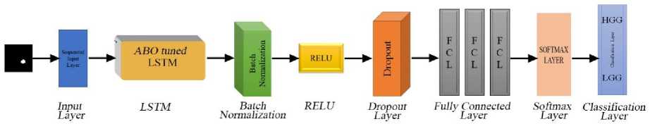
Fig.4. AOHLN network

The results of the LSTM layer is fed to the batch normalization layer which normalizes the output to stabilize and speed up the training. It adjusts the mean and variance of the data, ensuring consistent input distribution across layers. The normalized output is computed as in (29):

z t =

h j -M

V^2+^

where h_t is the input from the previous layer, ц is mean of the input, n ² is the variance of the input and r is a constant to ensure numerical stability. The Rectified Linear Unit (ReLU) function is then applied to introduce non-linearity, enabling it to capture complex data patterns. The ReLU function is defined in (30) as:

ReLU(z) = max(0, z)

where z is the input to the activation function. This function ensures that negative values are set to zero while positive values remain unchanged. LSTM output is passed through three sets of batch normalization and ReLU layer. A dropout layer is incorporated into the network to avoid overfitting by randomly turning off a fraction of neurons during training. This mechanism forces the network to generalize better by minimizing dependency on specific pathways. The dropout rate is set to 0.6, to balance regularization and effective learning.

The network includes three fully connected layers that progressively minimizes the dimensionality of the features extracted by earlier layers. This progression ensures that only the most relevant information is retained for classification. The final fully connected layer maps these features to the class scores as shown in (31).

z = W ■ h + b

where W - weight matrix, h -input vector and b is bias. A softmax layer then transforms these scores into class probabilities, enabling the network to predict the likelihood of each input belonging to a particular class. The probabilities are used for final classification and the network computes the loss using a cross-entropy function to guide its optimization process during training. Equation (32) and (33) shows the equation for softmax layer and classification layer loss function respectively.

P(yd =

e^z l

x^

L = -;ZL[y t log(y i ) + (1 - yd log ⁽ 1 - y i )^]

An auction-based optimization stage is incorporated to refine the LSTM classifier weights following initial training, with the objective of improving convergence stability and generalization. This meta-heuristic search helps the network avoid shallow minima and reduces classification variance. The overall focus of the framework remains on reliable tumor segmentation and classification, rather than on proposing a new optimization paradigm .

4.    Results and Discussions

The model, which includes DA-AtraDense U-Net for brain tumor segmentation and AOHLN for classification is evaluated here. The evaluation is based on quantitative metrics, visual comparisons and a comparison with existing methods. The BraTS2019 and BraTS2020 datasets, having high-grade gliomas (HGG) and low-grade gliomas (LGG), are used for validation. This method was developed using MATLAB. The system used Windows 11 64bit operating system on Ryzen™ 5 5600H processor operating at 3.30 GHz, with 8 GB of RAM.

For tumor segmentation performance, the Dice Similarity Coefficient (DSC) and Jaccard Index (Intersection-over-Union, IoU) are used as the primary evaluation metrics, as they directly assess the spatial overlap between the predicted and reference tumor masks. For tumor classification, a comprehensive set of diagnostic metrics is considered, including Accuracy, Sensitivity (Recall), Specificity, Precision, F1-score, False Positive Rate (FPR), False Negative Rate (FNR) and Matthews Correlation Coefficient (MCC), to provide a balanced and reliable assessment of diagnostic performance.

The segmentation accuracy of the developed method is evaluated using the DSC which assesses the overlap between the actual and predicted tumor regions and IoU, which provides a detailed measure of how well the predicted segmentation matches the ground truth. DSC and IoU are the most appropriate measures for tumor segmentation in highly class-imbalanced BraTS MRI data. Since background pixels dominate brain MRI scans, pixel-wise accuracy can be misleading, because even a model predicting only background can yield very high accuracy.

Input

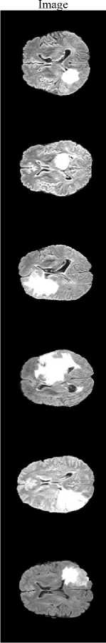
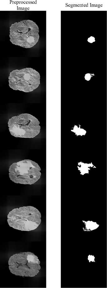
Fig.5. Segmented Image using proposed system

The proposed method achieves a DSC of 0.9907 and a Jaccard Index of 0.9816, demonstrating excellent agreement with expert annotations and confirming that the framework precisely localizes and segments the tumor region rather than over-predicting background. Fig.5 illustrates the segmentation results, where the tumor regions are accurately delineated from the surrounding brain tissues.

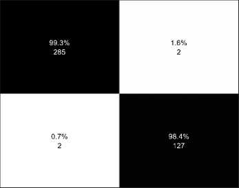
Table 1 shows the hyperparameters used in the classification stage of the proposed system. These hyperparameters were able to fine tune the system to achieve a higher accuracy in classifying the output as HGG or LGG. The classification of MR Images into HGG and LGG is performed for both the BraTS datasets. Fig.6(a) shows the confusion matrix of BraTS2019 dataset and Fig.6(b) shows the confusion matrix of BraTS2020 dataset. For testing 259 HGG images and 76 LGG images were used from BraTS2019 dataset. And 287 HGG and 129 LGG images were used for testing from the BraTS2020 dataset. In the case of BraTS2019, 256 HGG and 75 LGG images were predicted correctly and in BraTS2020 dataset, 285 HGG and 127 LGG images were correctly predicted by the proposed method. The accuracy obtained by the proposed system for BraTS2019 dataset is 98.81% and for BraTS2020 is 99.04% respectively.

Table 1. Hyperparameter used for classification

Sl.No	Parameters	AOHLN
1	Initial learning rate	0.001
2	Mini batch size	32
3	Max epochs	100
4	Hidden Units	100

The performance parameters of the proposed method is evaluated for different metrices and a comparison of the parameters for both BraTS2019 and BraTS2020 datasets is provided in the table 2. From the table 2 it can be viewed that the proposed model gives a better performance with BraTS2020 dataset in terms of accuracy, F1 score, sensitivity and Matthews Correlation Coefficient (MCC) whereas the precision and specificity for BraTS2019 dataset is higher than BraTS2020 dataset for the model.

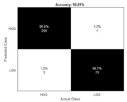
(a) BraTS2019

Fig.6. Confusion matrix of the proposed system

Accuracy: 99.04%

HGG                   LGG

Actual Class

(b) BraTS2020

Table 2. Performance parameters of the proposed system

Parameters	BraTS2019	BraTS2020
Accuracy	98.81	99.04
Sensitivity	98.84	99.30
Specificity	98.68	98.45
Precision	99.61	99.30
F1 Score	99.22	99.30
Matthews Correlation Coefficient	96.64	97.75

Based on the datasets, this section provides a detailed comparison of the suggested method's performance against other existing DL models, such as CNN, LSTM, ResNet and DCN. Accuracy, precision, sensitivity, specificity, F1 score, false positive rate (FPR), false negative rate (FNR) and Matthews correlation coefficient (MCC) are among the metrics used to assess performance.

The results presented in Table 3 shows that the evaluation of developed method outperforms when compared to the existing methods on the BraTS2019 dataset. It has achieved the highest accuracy at 98.81%, outperforming CNN (96.12%), LSTM (97.01%), ResNet (97.91%) and DCN (98.21%). This demonstrates the method's efficiency in handling complex brain tumor classification tasks. The suggested method has achieved the highest precision of 99.61%. than any of the models evaluated. Similarly, it has the highest sensitivity (98.84%) and specificity (98.68%), indicating a balanced ability to correctly classify both positive and negative cases. The proposed method achieves the highest F1 score of 99.22%, demonstrating an excellent balance of precision and recall. Furthermore, it has the lowest FPR (1.32%) and FNR (1.16%), demonstrating its effectiveness in reducing misclassification rates. MCC value of 96.64% further highlights the strong correlation between the predicted and actual classes.

Table 4 shows the performance on the BraTS2020 dataset, which emphasizes the proposed method's robustness. It achieves 99.04% accuracy, outperforming CNN (96.88%), LSTM (97.12%), ResNet (97.6%) and DCN (98.32%). With a precision of 99.3% and a sensitivity of 99.3%, the proposed method excels at correctly identifying tumor cases. It has a specificity of 98.45% which ensures that non-tumor cases are correctly classified, lowering the risk of false alarms. The suggested model also outperforms the existing models in all other parameters too.

Table 3. Performance parameters comparison for BraTS2019

Parameter	CNN	LSTM	ResNet	DCN	Proposed
Accuracy	96.12	97.01	97.91	98.21	98.81
Precision	98.43	98.82	99.22	99.22	99.61
Sensitivity	96.53	97.3	98.07	98.46	98.84
Specificity	94.74	96.05	97.37	97.4	98.68
F1 Score	97.47	98.05	98.64	98.84	99.22
FPR	5.26	3.95	2.63	2.6	1.32
FNR	3.47	2.7	1.93	1.54	1.16
MCC	89.27	91.7	94.16	95	96.64

Table 4. Performance parameters comparison for BraTS2020

Parameter	CNN	LSTM	ResNet	DCN	Proposed
Accuracy	96.88	97.12	97.6	98.32	99.04
Precision	97.9	98.59	98.6	98.95	99.3
Sensitivity	97.56	97.21	97.91	98.61	99.3
Specificity	95.35	96.9	96.9	97.67	98.45
F1 Score	97.73	97.89	98.25	98.78	99.3
FPR	4.65	3.1	3.1	2.33	1.55
FNR	2.44	2.79	2.09	1.39	0.7
MCC	92.71	93.34	94.41	96.08	97.75

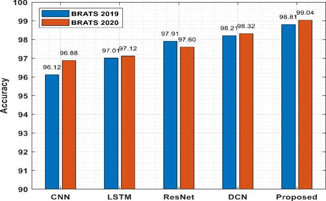
Fig.7. Accuracy comparison with existing models

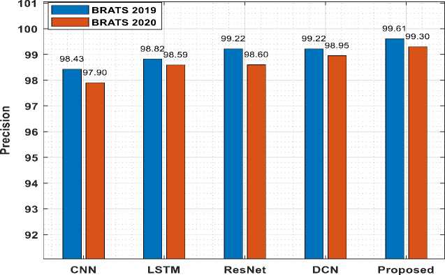
Fig.8. Precision comparison with existing models

Fig.7 shows the accuracy comparison of suggested model for both dataset with the existing algorithms. From Fig.7 it can be inferred that the proposed model produces higher accuracy and also the processing of BraTS2020 MRI images gives higher accuracy. Also, Fig.8 displays the precision comparison of proposed model for both datasets with the existing methods. Precision for BraTS2019 dataset is comparatively higher when compared with BraTS2020.

The computational performance of the proposed framework was evaluated and the average pre-processing and segmentation time was 13.33 seconds, while feature processing and classification (including feature extraction, feature selection and AOHLN inference) required 84.91 seconds. The total end-to-end computation time required was 98.24 seconds. These results indicate that the classification and feature-processing stage accounts for the majority of the computational cost, whereas segmentation contributes a comparatively smaller overhead. Although real-time operation is not achieved in the present CPU-only implementation, the runtime remains practical and further latency reductions are expected with GPU-based deployment and model optimisation. Table 5 shows the average computational performance for the proposed system.

Table 5. Computational time analysis

Processing Stage	Average Time (s)
Pre-processing + Segmentation	13.33
Feature Processing + Classification	84.91
Total Runtime	98.24

To assess the stability and generalisability of the proposed classification framework, a 5-fold cross-validation strategy was employed on both the BraTS2019 and BraTS2020 datasets. The data were partitioned and performance metrics were averaged across the five folds. The proposed method achieved a mean accuracy of 98.45 ± 0.39% on BraTS2019 and 98.66 ± 0.27% on BraTS2020, together with consistently high precision, sensitivity, F1-score and MCC values as shown in table 6. The narrow standard-deviation ranges demonstrate that the model performance is stable across different folds and is not dependent on a single train–test split.

Table 6. 5-fold cross validation performance of the porposed system for BraTS2019 and BraTS2020 data

Metric	BraTS2019	BraTS2020
Accuracy	98.45 ± 0.39	98.66 ± 0.27
Precision	99.06 ± 0.44	99.02 ± 0.29
F1-Score	98.99 ± 0.25	99.02 ± 0.20
Sensitivity	98.91 ± 0.17	99.02 ± 0.29
Specificity	96.92 ± 1.42	97.83 ± 0.64
MCC	95.65 ± 1.07	96.86 ± 0.64

An ablation study was carried out to assess the individual contribution of each stage in the proposed framework, namely pre-processing, segmentation, radiomic feature extraction, feature selection and classification using BraTS2019 dataset and is shown in table 7. When only pre-processing and direct classification were applied, the system achieved 92.84% accuracy. Incorporating tumor segmentation increased performance to 96.12%, confirming the benefit of restricting analysis to the tumor region. The addition of KED–GLCM radiomic features further improved accuracy to

97.31%, demonstrating the value of explicit texture and edge-based heterogeneity modelling. Finally, CMO-based feature selection yielded the highest performance at 98.80% accuracy and 96.64% MCC. These results show that each module contributes incremental performance gains and collectively leads to the best overall outcome.

Table 7. Ablation study of the proposed system

Preprocessing	Segmentation	Feature Extraction	Feature Selection	Classification	Accuracy	Precision	F1 Score	Sensitivity	Specificity	MCC
Yes	No	No	No	Yes	92.84	95.33	95.33	95.33	84.62	79.95
Yes	Yes	No	No	Yes	96.12	97.28	97.47	97.66	91.14	89.19
Yes	Yes	Yes	No	Yes	97.31	98.83	98.26	97.7	96	92.4
Yes	Yes	Yes	Yes	Yes	98.8	99.61	99.22	98.84	98.68	96.64

Fig.9 displays the accuracy comparison of the previous related works with the current method. Saeed Iqbal et al. achieved an accuracy of 97.5% using FusionNet [13] and Atika Akter et al. used CNN and U-Net model to classify brain tumors with 97.7% accuracy [14]. SM Alqhtani et al. classified tumors with 98.2% accuracy using FCM-SVM model [19], while Rajeev et al. [24] achieved an accuracy of 98.4% using hybrid EBiLSTM and S Natha et al. [18] obtained 98.7% accuracy using SETL-BMRI model. The proposed DAAtroDenseU-Net-AOHLN method has achieved an overall accuracy of 98.99% for classifying tumors.

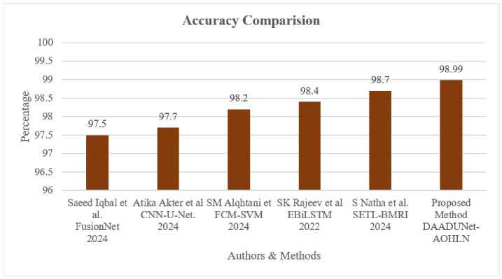
Fig.9. Accuracy comparison of proposed method with previous related works

The improvements in accuracy, precision and F1 score highlight its capacity to extract key features and perform effective classification. Moreover, the low false positive rate (FPR) and false negative rate (FNR) demonstrate its robustness in minimizing classification errors, a critical factor in medical applications where accuracy is crucial. The proposed method's steady performance across both datasets highlights its generalizability and dependability. Compared to traditional models like CNNs and LSTMs, the proposed method employs advanced architectural improvements, leading to higher performance. Its ability to surpass complex models such as ResNet and DCN further confirms its usefulness in addressing difficult classification challenges. It is also acknowledged that nnU-Net [32] currently represents a widely adopted benchmark framework for BraTS tumor segmentation. The present work is focused on developing and analyzing the proposed dual-attention AtroDense U-Net–based framework rather than on direct competition with nnU-Net challenge submissions and a detailed comparative evaluation with nnU-Net is considered an important direction for future work.

The proposed framework also has the potential to be integrated into AI-assisted radiology workflows. The system can automatically segment the tumor region and generate classification output in the background, providing decisionsupport to the radiologist rather than replacing clinical judgement. With further validation on clinical data, the method may assist in faster image review and more consistent reporting in neuro-oncology practice. The proposed framework demonstrates strong performance on the BraTS datasets, but it remains dependent on high-quality annotated data for both training and evaluation. The BraTS datasets are curated and may not fully reflect variations in scanner type, field strength, acquisition protocol or clinical image quality. Further validation on multi-center real-world data is required to confirm the generalizability of the method. In addition, real-time deployment testing was not performed in this study and system latency remains an area for future optimization.

DL models can learn latent representations, the DA-AtroDense U-Net in this work is primarily designed for accurate tumor segmentation rather than grading. Handcrafted texture features such as Kirsch and GLCM are extracted only from the segmented tumor regions to explicitly capture spatial heterogeneity and intensity variations that are critical for distinguishing HGG and LGG tumors. This hybrid design improves robustness and interpretability while adding minimal computational overhead, since feature extraction is confined to the tumor area.

5.    Conclusions

Brain tumors pose a serious health concern and accurately segmenting and classifying them is vital for proper diagnosis. Tumor complexity and variability continue to make these tasks highly challenging. A reliable and precise solution to the critical task of brain tumor diagnosis is provided by the suggested dual-stage framework, which combines DA-AtroDense U-Net for brain tumor segmentation and Auction-Optimized Hybrid LSTM Network (AOHLN) for classification. By integrating dual attention mechanisms, atrous convolutions and light dense blocks, the segmentation stage guarantees accurate tumor boundary localisation in MRI images. Even in intricate and diverse tumor regions, the model's capacity to acquire appropriate information and minute details is improved using the DA-AtroDense U-Net. Using the Auction-Based Optimisation (ABO) algorithm's optimisation power and LSTM's temporal feature extraction capacity, AOHLN effectively classifies the segmented tumor regions into the appropriate categories during the classification stage. Experiments on the BraTS2019 and BraTS2020 datasets demonstrated strong performance in both segmentation and classification. The model achieved a Dice Similarity Coefficient of 0.9907 and Jaccard Index of 0.9816 for tumor segmentation and overall classification accuracy of 98.99%, together with high precision, sensitivity, F1-score and MCC. The system not only enhances diagnostic accuracy, but also has the potential for clinical integration, allowing radiologists to make more informed decisions and streamlining the diagnostic process for brain tumors.

Future research can explore the application of this framework to multi-modal medical imaging data and real-time diagnostics and additional optimization of computational efficiency, further advancing its utility in healthcare applications.

Acknowledgment

Declaration of Competing Interest

The authors declare that they have no competing interests related to this work.

Data Availability Statement

Images     used     in     the     work     is     openly     available     in     Kaggle     website             (BraTS2019)             and (BraTS2020)