A Novel Method to Solve a Class of Non-local Diffusion Optimal Control Problems by using Bernstein Polynomials

Published Online June 2020 in MECS

Heat conduction equation is a famous partial differential equation in sciences. The classical parabolic heat conduction equation is shown as follows:

∂ w + λ ∆ w = h               (1)

∂t where w(x,t) shows the temperature in the position x and time t, λ is a constant coefficient, h(x,t) is a given continuous and well-behaved function, and Δ denotes the Laplace operator. The study concerning the heat conduction equation is returned to Fourier’s studies about heat conduction. In the last decades, the investigation of the unsteady heat conduction equation is increased. Initially, Morse and Feshbach [1] and then Maxwell [2] formulated some of the unsteady heat conduction equations. In 1959, Carslaw and Jaeger [3] and in 1969, Rotem and Neilson [4] considered the repercussion of heat conduction equations. In 1971, Tamir and Taitel improved work’s Rotem; see [5]. In 1972, Taitel presented a solution for a thing with a thin layer by parabolic, hyperbolic, and discrete heat conduction equations (see[6]). By using his work and other scientists, the application of heat conduction equation in the analysis of phenomena and physical processes such as industrial process, long cylinder, and plan wall was incremented. In the recent decade, wise methods for solving this problem have increased. Pavlov and Kudoyarova [7] solved this problem with the Spline method. Al-Khaled [8] used the Fourier regularization method. In many books and articles for solving the heat conduction equation, the finite element method was used (see[9,10,11]); many authors solved this problem by the Meshless method (see[12,13] and references therein).

In recent years, Bezier functions have attracted the attention of researchers. These functions are suitable tools for solving partial differential equations (PDEs) as a meshless method, and also these tools have excellent properties such as a straightforward definition, quick in determination and execution in the computer, continuity property interpolation end-points and symmetry property.

Bezier functions were applied for solving Fredholm integral equations (see[14,15,16]), Volterra integral equations [17], and Volterra–Fredholm–Hammerstein integral equations [18]. Zheng et al. [19] and Safaie and

Farahi [20] introduced the Bernstein–Bezier form for solving ordinary differential equations and they used an objective function based on the Bezier control points. In this paper, we consider optimal control problems governed by the nonlocal diffusion equation using Bernstein polynomials. To obtain the optimal pair of trajectory and control functions, we use the operational matrices of derivative and integral and then solve the optimal control problem by converting PDE constraints to an algebraic system.

The remainder of this paper is planned as follows: Section 2 introduces some essential properties of Bernstein and Bezier functions. In Section 3, we consider the one-dimensional diffusion equation with initial and boundary conditions and then, by using Bezier function, convert this one-dimensional diffusion equation to a mathematical optimization problem. In Section 4, we convert this problem to a quadratic programming problem with linear constraints and also remind four issues for solving the problem. In Section 5, we give the convergence analysis of the present method. In Section 6, three numerical examples are solved, which show the efficiency and reliability of our method. A conclusion is given in section 7.

• II.    Preliminaries

Bezier curves have more interesting properties than the cubic or B-splines. For example, in the cubic spline, if we change only two interpolating points, then we need to redetermine the cubic spline function, but in Bezier functions, one can find a new Bezier function from the old one. Bezier functions are used in computer-aided design (CAD) (see[21]), computer graphics to draw shapes, solving the various control problems such as switching control systems (see[22]), and many different applications (see[23,24,25,26,27,28,29]).

This section consists of some basic definitions and properties of Bezier functions.

Definition 2.1 The Bernstein polynomials of degree n over the interval [0,1] are defined as follows:

n

Bn (t ) = I    It (1 -t) n— i к i J for i = 0,1,2,..., n where ( n 1 = —n!—.

к i J    i !( n — i )!

If one uses the binomial expansion for (1—t)n—i, then n—i

Bi (t ) = Zin, i )(n I (—1) kf+k(2)

k=0 к k J к i J then the Bezier polynomial of degree n over the interval [0,1] is defined as follows:

Pn (t ) = Сфп (t)(3)

where

C = [ Co  C1   • " Cn ]

is the vector of constant coefficients that we recall its entry as control points. Thus ( 3 ) and ( 4 ) implies that

n

P , ( t ) = Z B ( t ).

i =0

Lemma 2.3 By using (2), we define ф ( t ) = ф T_n ( t )

where T ( t ) = [ 1 t ••• tⁿ J T and y_n = T ^{n + 1} is an ( n + 1) x ( n + 1) upper triangular matrix that can be expressed by

( — 1) j ^— i n !

XI/ ^{n + 1}     ₌ I

^T i + 1, j + 1

^{( n —} j ^)!( j ^— i ^{)! i} !,

0,

for i , j = 0,1,   , n .

Proof. See [30].

Lemma 2.4 Suppose that H = L ² [0,1] and that { B n ( t ), B n ( t ),..., B n ( t )} c H , and let Y = Span { B 0 ⁿ ( t ), B 1 ⁿ ( t ), , B n ⁿ ( t )}. Y is a finite-dimensional subspace of the complete space L ² [0,1] , and it is a complete basis for the Hilbert space H .

Proof. See[31].

Definition 2.5 Let X= (X, . ) be a normed space and let Y be a subspace of X. Given a point x e X, a point y e Y is called a best approximation to x out of Y if y has the minimum distance from x. The problem of determining such a point is called the best approximation problem.

Ramark 2.6 If f (t) e L2[0,1] and Y = Span{Bn(t), Bn(t), ,Bn(t)} , then the best approximation of order n of the function f(t) in [0,1] is unique and is given by P(t) where f (t)^ Pn (t) = СФп (t),

Definition 2.2 Define a Bernstein vector ф_п ( t ) as ф , (t ) = [ B n ( t )   B n ( t )     •  B n ( t ) ] T ;

and C is completely dependent on f ( t ) . In fact C can be obtained by

C = <  f (t ) V ( t ) > Q - 1

where

< f ( t \ф„ ( t ) > = J f ( t V (t ) dt

= [          ], and the entries of the (n +1) x (n +1) matrix Q are defined as follows:

^Q = <  V n ⁽ t ), V n ⁽ t ) > = J X ⁽ t V T ⁽ t ) ^dt

= [> Л ( t )) V T ( t )) T dt             (5)

= V n J T ⁽ t^)T T ⁽ t ) ^dt V T = Y n G^ V ^ 0

where  Gn is the following (n +1) x (n +1) Hilbert matrix [31,32]:

	1	1	1	1    "
		2	3	n + 1
	1	1	1	1
Gn =	2	3	4	n + 2
		1	1	-^.
	[ n + 1	n + 2	n + 3	2 n + 1 ]

Theorem 2.7 Let f (t ) e C m [0,1]; that is f and all its derivatives up to order m are continuous and differentiable on [0,1] and let Y = Span { B 0 ⁿ ( t ), B 1 ⁿ ( t ), , B n ⁿ ( t )}. If P n ( t ) is the best approximation of f out of Y , then the mean error bound is

II f ( t ) - P n ( t Ж <

2 M

( m )!л/2 m + 1

where M = max | f ^{( m )} ( t )| .

Proof. We consider the Taylor polynomials f (t) = f (10) + f’(to)(t -10) + f"(10)(t-t°f m-1

+ ...+ f^{(m - 1)} ( t ₀)(---- 0 )—,      t , t ₀ e [0,1],

⁰   ( m - 1)!           ⁰

which we know that there exists f e [0,1] such that

m i f (t)- f (t )|=|f(m’сж —°)- .

m !

Since P(t) is the best approximation of f , so we have

II f ( t ) - P n ( t )||₂²<| f ( t ) - f ( t )|| 2

1                     ,1 (          A-tA” A²

=[ i f(t)-f(t) |2 dt=j 11 f(m>(f) ।(—o^- I dt i0                               JO i                     ”! I

• _<   2 M ² S^{(2 m + 1)}  _<      2 M²

• " [ ( m )! ] 2 (2 m + 1) "  [ ( m )! ] ² (2 m + 1)

where S = max{ 1 - 1 ₀, t ₀}.

Theorem 2.8 Suppose that f(t ) e C m [0,1]; then for each k e N ,   k <  m , and k <  n , there exists an

( n + 1) x ( n + 1) matrix D_B  such that

n

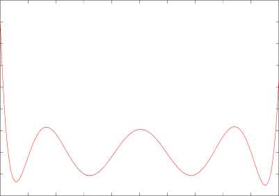
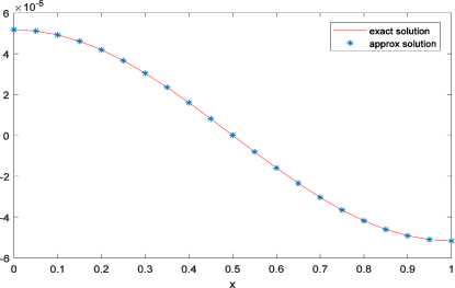
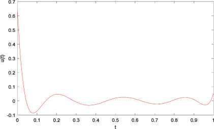
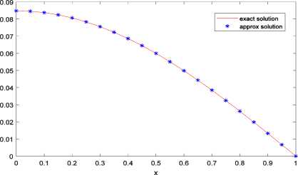
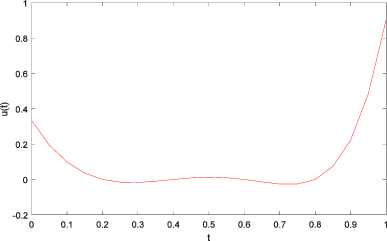
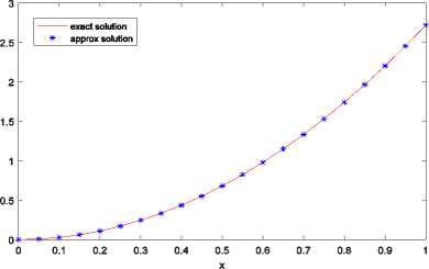
k f

where DB = vnAV, with f i,   i = j +1, i+1, j+1    [0  otherwise, for i = 0,...,n and j = 0,...,n-1 and V can be expressed by

• v_: = V-k,    ^k = ^1,2,•••^{, n}

where Y-k is kth row of V^-.

Proof. See [33].

Theorem 2.9 Let P_B be an (n +1) x (n +1) matrix; then

LxVn⁽t)^dt = ^PB V⁽x)               ⁽⁷⁾

0n where

Ps = wns, n and     is defined as:

w = [yv  И2  - и;+1 ]T such that

(-1)^n-i

i

Mi =[0 0  ... 0  (-1)⁰

The (n +1) x (n +1) matrix П is defined as

100   0

П =

^{n + 1}- (n+1)x(n+1)

and the matrix    is defined by

U=-£-

2 n + 2

( 2 n +1^

( 2 n + 1J

and the elements of Q are defined as

^Q( i+1)( j+1)

i, j = 0,1,   ,n.

The matrix P is called the operational matrix of integration.

Proof. See [34].

Now assume that w(x,t) is a function in a two-dimensional defined space on [0,1] x [0,1], and suppose that ф (x) and ф_п (t) are Bernstien vectors of degree n over the interval [0,1]; then we can approximate w(x,t) as follows:

^w(x,t) ~ ^^rnjB”⁽x)Bn(t) = ф„^г (x)Мф„(t) i=0 j=0

where

r m,. m 21 m12 m1n m1 n+1 " m 2 n+1 Mw = mn 1 mnn+1 (8) _ mn+11 mn+12   • ••   mn+1 n mn+1 n+1 - and m , i, j = 0,1, 2,  ,n, are constant numbers which are called control points. We describe later how one can find these control points.

• III.    Problem Statement

Now, due to (1), we consider the one-dimensional diffusion equation:

wt (x, t) - Awxx (x, t) = h(x, t),  (x, t) e (0,1) x (0,1)(9)

with the initial and boundary conditions as follows:

w(x,0) = f (x),  x e [0,1](10)

w(0, t) = g(t), t e [0,1](11)

and the nonlocal boundary condition

J w(x, t)dx = u (t)

where h(x, t), f (x) and g(t), for x e[0,1] and t e [0,1], are given continuous and well-behaved functions. The parameter X is a given constant number.

We are going to find the control function u(t) such that

w(x,1)=F(x)               (13)

where  F(x)  is a given continuous function for x e [0,1].

The control function u(t) will be termed admissible if it is a measurable function on [0,1] and the solution of the partial differential equation (9) satisfies the initial and boundary conditions (10)-(12) and also the terminal condition (13) holds.

The classical optimal control problem consists of finding an admissible control u(t) which minimizes the functional

J(u) = J*||u(t)||²dt.                (14)

Non-local diffusion equation (9)-(11) arises in many scientific and engineering applications such as atmospheric pollution controls [35]. Efficient methods to solve diffusion equations are important in successful applications of these kind of problems. There are some methods in solving such problems (see[36] and reference therein). The present paper extends for the first time, the using of Bernstein’s approximation in solving non-local diffusion optimal control problems.

To solve the optimal control problem (9)-(14), by using Bezier functions, one may convert the optimal control problem to a mathematical programming problem subject to algebraic equations.

According to the previous section, we assume that

w(x, t) ~ фФ (x)MwPn (t)

and that

u(t)^ ^.B, (t) = Mu^, (t)(16)

i=0

where

Mu = [ u1 u 2 u3  • " un+1 ]

where m_y ’s and u_k’s, i, j,k = 1,...,n +1, are control points that need to be found. By applying (15) and (16), one can easily find that

w⁽x,0) ~ ф,⁽x)MV,⁽⁰⁾,

w(0, t)^ ф, (0)M_wVn (t),

w(x,1) ~^T (x)MwVn(1), wt (x, t) - ФП (x)MwDB Фп (t), wx(x, t)  Ф, (x) D^Mw^, (t), wxx (x, t)  Ф, (x)D^ DBn MwVn (t),

J ‘^w(x, t)dx^P Ф,⁽1)MV,⁽t)• 0n

We recall that the matrix D is defined in (6), and for J^w(x, t)dx, we use (7).

Similarly for J , we have

J⁽u ) = Cl l^{u (}t )|Г ^dt- С ^{[ М}иФп⁽t )Ф^{Т (}t)M^T ] ^dt   z_1Cx

⁰⁰       (18)

TT

UT n пт n u where G is given in (5).

Now the optimal control problem (9)-(13) with cost functional (14) can be approximated by the following optimization problem:

minimize   J = Mт_п GTT MT     (19)

such that

Фп⁽x)^Mw^DB_nФп⁽t) — Фп I x)DBT MwVn (t) = h(x, t),

Фп (x)MwVn (0) = f (x), фПТ (0) Mw^n (t ) = g (t),                             (20)

Ф, (1)P/ Mw^n (t) - MuФп (t) = 0,

Фп⁽x ) ^Mw^n⁽¹⁾= F⁽x )

where x, t e [0,1] and the matrix  M_w         and

( n+1)x( n+1)

vector M_u of order n +1 are unknowns. By solving the problem (19)-(20) one can find the matrix M and the vector M . Thus by (15) and (16), it is possible to find the best approximation of functions w(x,t) and u(t), respectively. In the next section, we precisely describe how one can solve the optimization problem (19)-(20).

• IV.    Solving Optimization Problem

Let r,s eZ⁺. Choose x_t ’s (i = 0,...,r) and t_y ’s (j= 0, ,s) nodes on the interval [0,1]. Using these nodes in conditions (20), that convert these constraints into a algebraic system with (s +1) x (r +1) linear equations and (n +1) x (n +1) + (n +1) unknowns as:

Aij    = bij where by (8) and (17), TT     T    T    T

LMwо  Mw1  *" Mw(n-1)  Mwn Mu J , and bij = [h(xi,tj)   f (xi)   g(tj)   0   F(xi)]T, and Atj is a 5 x (n +1)(n + 2) matrix defined by discrete equations (20) for every i e {0,...,r} and j e {0,...,s}.

Now we solve a quadratic programming problem to find     (in other words, M and M ):

The algorithm of this method is as follows:

INPUT: n, rand s.

• >Calculate D_n and P , operational matrices of

derivative and integral.

• >Set M_w  and M_u, control points matrix and

vector for w(x,t) and u(t),  respectively.

• >For i = 0 to r and j = 0 to s do: Compute

A   and  b ,  for the linear constraints of problem.

• >    Solve the following quadratic programming problem to find M and M .

minimize J = M_uT_nG_nT^TMu^T

Such that A =b , i = 0,1,   ,r,   j = 0,1,   ,s.

OUTPUT: w(x, t) ^ фТ(x)MwФn (t), u(t) ^ MuФn(t), and cost function J.

By using different optimization tools, this optimization problem can be solved by many useful computational softwares such as MATLAB. We need to remind

• •    x= t= 0and x= t=1 .

• •    Generally x ’s   (i= 1,   , r- 1) and t ’s

• ( i= 1,   , s- 1) are not equal in lengths.

• •    If the solution is undesired, then we may increase r ors (the number of nodes) or n (the degree of Bezier function).

• •    The (n+1)×(n+1) matrix ψGψ^T is symmetric positive definite.

  (22) and

  
  

V. Convergence Analysis

In this section, we provide a theoretical analysis about the convergence of above method. Without loss of generality, for the functional J in (14) , consider II u(t) II2=u(t)uT(t) . Also for simplicity, consider λ=1. Summing two relations (9) and (12), we have w (x, t) -w (x, t) +  w(x, t)dx-u(t) = h(x,t).

t              xx             ₀

We prove the convergence by the degree raising of the Bezier functions approximation when the control-point-method is applied to the following optimal control problem:

∫1T u(t)u (t)dt subject to

L(w(x,t),w_t(x,t),w_xx(x,t),u(t)) = w_t(x,t)

-w (x, t) + ∫ w(x,t)dx-u(t) = h(x,t)

where     w(x,0) = f (x),    w(0, t) = g(t)    ,

w(x,1) = F(x) .

Definition 5.1 Let Ω= [0,1]×[0,1] and let р={Bⁿ(x)B^m(t)|0≤i≤n,0≤ j≤m}⊂L²(Ω) be the set of Bernstein polynomial products when n,m∈N∪{0} . We define B as B = Span{р}.

Theorem 5.2 Let P be the best approximation of f∈L2(Ω) in Bnm. If snm(f)=   | f(x,t)-Pnm(x,t)|2dΩ,

Ω then lim  snm(f) =0.

(n,m)→(∞,∞)

Proof. See [37].

Theorem 5.3 Under the stated assumptions Theorem 5.2, the approximate solutions B =ϕ^T(x)M ϕ(t) and u = M ϕ (t) , convergence, respectively, to the exact solutions w^*(x, t) and u^*(t) in the optimal control problem (22)-(23) when (n,m) → (∞, ∞) .

Proof. Let 6 >0 and let (x, t) ∈[0,1]×[0,1] . By using Theorem 5.2, we can easily find the Bernstein functions P        and      w       such     that     and nm                     n

w^*(x,t)-P_nm(x,t) ≤,

IIu^*(t)-w_n (t) ≤.

By assuming n and m sufficiently large, it is easy to find that

IIf(x)-Pnm(x,0) ≤,

IIg(t)-Pnm(0,t) ≤,

F(x)-Pnm(x,1) ≤.

But perhaps P  (x, t) and w(t)  do not satisfy precisely in the initial and boundary conditions. So we define B   (x, t) as follows:

B_nm (x,t)=P_nm (x,t)+xtα(x)+xβ(x)+γ(t)

such that this new function satisfies the initial and boundary conditions, that is,

Bnm(x,0)=f(x),

Bnm(0,t)=g(t),

Bnm(x,1)=F(x).

According to (23), we have

II f(x)-Pnm(x,0)II⁼xβ(x)+γ(0) II≤,

IIg(t)-Pnm(0,t) = γ(t) ≤,

F(x)-Pnm(x,1) = xα(x) + xβ(x) +γ(1)≤.

Since xβ(x) II - γ(0) II≤II xβ(x)+γ(0) ≤    , xα(x) - II xβ(x)+γ(1) ≤ xα(x) + xβ(x) +γ(1)≤,

J(u) =  ¹  u(t) ²dt

en = max | w(x,1)- w(x,1)| i g{0,..., r }

such that wt (x, t) - Wxx (x, t) = 0,   (x, t) G (0,1) X (0,1), wx(0,t) =u(t), wx (1, t) = 0,      w( x, 0) = cos (nx)

where the function . indicates the Euclidean norm. We are going to find the admissible control function u(.) such that the solution of the above partial differential equation corresponding to the given boundary conditions satisfies the following terminal condition:

w( x, 1) = cos (nx) exp(-n2), where w(x,1) indicates the approximate solution of the diffusion equation at the final time t =1 .

Table 1. The absolute error in Example 1.

Degree of Bezier polynomial (n)	Absolute error (e )
10	2.1266 x10"12
11	2.6110 x10"15
13	2.1460 x10"17
15	1.9590 x10-17
16	1.3922 x10"17

Fig.1 and Fig.2 show the approximated graphs of control and terminal condition w(x,1) .

The exact solution is     u(t) = 0     and

w(x, t) = cos(nx)exp(-n21) . By using the Bezier function, we expect u (t ) = MuVn (t )-0

and wx,t) = ^T (x)MwVn(t) - cos(nx) exp(-n21).

For n = 8, the control is found as u (t) ~ 6.0695 X10-9 Bo8( t) - 3.6448 x 10-8 Bv3( t)

+1.1633 x10^-7B₂⁸( t) - 2.2266 x10^-7B₃⁸( t)

+2.7047 x10^-7B₄⁸( t) - 2.1110 x10^-7B₅⁸( t)

+1.0286x10 'B68(t)-2.4404x10"2B78(t) + 3.2433x10-9B88(t), and the terminal condition is found as

w(x ,1)^5.1723 x 10"⁵B_o⁸(x) + 4.1379 x 10^-4B,⁶(x)

+1.1929x10^-3B₂⁸(x) +1.3657x10 3B₃⁸(x)

• -9.8504 x 10^-9B₄⁸(x) -1.3657 x 10^-3B₅⁸(x)

• -1.1929 x10^-3B₆⁸( x) - 4.1379 x10-* B₇⁸( x) - 5.1723 x10^-5B₈⁸( x),

  x10"⁹

  ³ 2

  -1

  -2

  

  0       0.1      0.2      0.3      0.4      0.5      0.6      0.7      0.8      0.9       1

  t

  Fig.1. The graph of approximated control

  
  
  

  Fig.2. The graphs of approximated and exact terminal trajectory w(x,1)

  
  

and

J = 9.6549 x10"¹⁹.

The absolute error of the exact solution and approximate solution given for different values of the degree of Bezier polynomials are shown in Table 1. The numerical results in this table show that the present method is convergence. To illustrate this aim, we define

Example 2

In the second example, we consider the one-dimensional diffusion equation (9)-(13), where (see [39]):

h (x, t) = 0,  f (x) = cos (^x),

п             n x     n g (t) = exp(-—t),  F (x) = cos (—)exp( - —).

Now we need to find u(.) and minimize the functional

J(u) = J„11 |u(t) II²dt.

By using the Bernstein polynomial of degree 8 , the control function is found as

u(t) ~ 0.6366Bo'tt)-2.5370B8(t) + 5.8914B27(t) -8.7804B32 (t) + 2.7012 B42 (t) - 5.7216 B52 (t) + 2.3956B67( t) -0.5706B72 (t) + 0.0540B87( t), and the trajectory w(x,1) is found as:

w(x,1) ~ 7.4705 x 10 2B_o²(x) + 7.4705 x 10 2B7 (x) +7.1067 x 10^-2B₂⁷(x) + 7.3595 x 10^-2B₃⁷(x) +6.2693 x 10^-2B₄⁷( x) + 4.7976 x 10 ' B₅²(x) +3.3303 x 10^-2B₆²(x) +1.6651 x 10^-2B₇²(x).

The cost function J is

J = 5.0070 x10^-3.

Table 2. The absolute error in Example 2.

Degree of Bezier polynomial (n)	Absolute error (e )
8	6.9440 x10"10
9	2.2657 x10"11
10	2.1517 x10-13
11	2.3004 x10"13
12	5.7024 x10-14

Fig.3 and Fig.4 show the approximated graphs of control and terminal condition w(x,1) .

Fig.3. The graph of approximated control

Fig.4. The graphs of approximated and exact terminal trajectory w(x,1)

Example 3

In this example, we consider the one-dimensional diffusion equation (9)-(13) where (see [40]):

h (x, t ) = ( x²- 2) e,    f (x ) = x²,

g(t) = 0,     F(x) = x²e.

Now we must find u(.) and minimize the functional

J⁽u) = J11 |u⁽t)H^{2 dt}.

The exact solution is u(t) = ^e and w(x,t) = x²e^t .

For n =8 the control of this problem is found as

u(t) ~ 0.3333B_o⁷(t)-0.7467B,⁷(t) -0.1095B₂⁷(t)

-0.0346B₃⁷ (t) + 0.1195 B₄⁷ (t) + 0.1179 B₅⁷ (t)

-0.1559B67 (t) - 0.3736B77 (t) + 0.9061B87 (t), and the terminal condition is approximated by

w(x,1) ~ 2.7173B27(x) +16.3097B37(x) +40.7742B42 (x) + 54.3656B52 (x) + 40.7742B67 (x) +16.3097B72( x) + 2.7173B82( x), and J = 10.1225 x10-3.

Fig.5 and Fig.6 show the approximated graphs of control and terminal condition w(x,1) .

Fig.5. The graph of approximated control

Fig.6. The graphs of approximated and exact terminal trajectory w(x,1)

• VII. Conclusion

In this paper, we introduced a new set of functions that are called Bezier functions for solving optimal control problems governed by a nonlocal diffusion equation with given boundary and terminal conditions. The method is general and easy to implement by using operational matrices. Operational matrices, together with the collocation method, were used to approximate solution of this kind problems. The convergence of the method was proved. Some numerical examples were given to illustrate that this method is efficient.

ACKNOWLEDGEMENT

We would also like to show our gratitude to the referees for their helpful comments and useful suggestions.