A Parallel Ring Method for Solving a Large-scale Traveling Salesman Problem

Published Online May 2016 in MECS

Traveling Salesman Problem (TSP) is NP -hard therefore, for large-scale problems, it is challenging to produce optimal solutions in a reasonable time. Many problems in integrated circuit manufacturing, scheduling, analysis and synthesis of chemical structures, logistic problems, robotics, etc. can be modeled and solved as TSP problems. A lot of research has been done on using various techniques to generate good quality solutions that are close to the optimal [14, 15, 16, 20, 22, 39, 40, 43].

Local heuristic approaches are one of the main approaches to obtain near optimal tours for large instances of TSP in a short time [28, 39]. Both discrete optimization [28, 29] as well as continuous optimization [30, 31, 32] methods are used to solve the Euclidean as well as non-Euclidean TSP.

Many existing heuristic solutions for solving TSP with n points have O(n2) or higher complexity hence they are not efficient for solving large-scale TSPs. Lin-Kernighan heuristic is based on “tour-improvement” – it accepts a given tour and modifies it to obtain an alternative tour of lesser cost [20]. Chained Lin-Kernighan heuristic improves an existing solution and it overcomes some drawbacks in local optimization algorithms [2]. Applegate et al. [1] have calculated the optimal solution for a 85,900-points TSP - the largest problem that is solved optimally until now. This experiment required nearly 136 years of CPU time. Well-known test-cases for large-scale TSP problems contain up to 107 points [24] but, until now, there are no optimal solutions found for such problems. Interesting results were achieved in the challenge usa115475 problem, started by Cook, that has 115,475 points [25]. This large-scale problem started by Cook was solved independently by Clarist, Helsgaun, and Nagata [26]. Although the tour length of the solutions presented by these three researchers is exactly the same and is equal to 6,204,999, the three tours are mutually different. This problem inspired us to find optimal solutions for such large-scale problems. Using the heuristic presented in this research, we generated a solution with length 6,205,118, which is 0.0019% worse than the solution presented independently by Clarist, Helsgaun, and Nagata.

There have been a number of studies of human performance on the TSP [33, 34, 35, 36, 37, 38]. It is quite certain that human subjects do not search the whole or even substantial parts of the problem space when solving the combinatorial optimization problems because of memory and cognitive processing limitations, in spite of massive parallel processing of brain. This means that human subject might be using a kind of abstraction of data in solving the TSP. Many researchers have shown that humans produce close-to-optimal solutions to TSP in a time that is (on average) proportional to the number of cities [34, 35]. Note that the TSP instances were small (less than 150 cities) when experimenting with human subjects. Motivated by the human vision system, more specifically the vision fovea, the authors in [14, 22, 35, 38] used hierarchical representation (pyramid) to achieve abstraction of the data (cities). The main processes in obtaining a hierarchical model are clustering methods using merging or division principles [41]. For example, the cities are merged into bigger and bigger modes (called clusters), then an initial tour solution on the modes is produced [14]. A splitting strategy could be followed as well. The whole data space is split over and over again into cells of cities, creating modes [22]. Afterward, a refinement on this initial solution is done on modes, mimicking a human fovea, until the tour contains all the cities, producing an approximate solution for the TSP. This strategy is in fact a divide-and-conquer strategy, which seems to be plausible, taking the limiting processing power and space limitation of human brain.

Some TSP algorithms can be executed in parallel by decomposing the given set of points into clusters [4, 5, 6, 7, 8]. Bazylevych et al. [7] have proposed a “Ring” method that merges the TSP solutions obtained from different clusters into a complete initial solution. The goal of the current research is to reduce the computing time by using a large number of parallel processors. The maximum speedup was achieved when the number of processors is equal to the number of clusters into which the given set of points is divided. The current research is an extension to the work of Bazylevych et al. [8] that used a single processor. In the current research, the experiments are conducted on a distributed system that consists of many processors (a maximum of 64 processors) running in parallel.

The rest of the paper is organized as follows. Section 2 focuses on the problem formulation. Section 3 describes the parallel ring method, including the decomposition of given points into clusters, solving the TSP for each such cluster to generate partial solutions, merging the partial solutions to generate a complete initial solution, and optimizing the complete initial solution. Implementation and experimental results are presented in Sections 4 and 5 respectively. Finally, conclusions are presented in Section 6.

• II.    Problem formulation

Given a set P = {p₁, p₂, …, p_N} of n points that are described by their coordinates p_i = (x_i, y_i), i = 1 to n and the Euclidean distance function dist: P×P → ℝ that defines the distance between any two points then the problem is to find out a closed route M , with minimal length L , that starts from a point and visits each and every point only once and returns back to the starting point.

If dist(p i , p j ) = dist(p j , p i ) then this problem is symmetric else it is asymmetric. The problem considered in this research is of symmetric type. The problem is a kind of Hamilton cycle problem – finding a cycle in an undirected graph that visits each vertex exactly once and have a minimal length. The main goal of the current research is to develop a methodology to find a high quality shortest solution by using a large number of parallel processors.

• III.    The parallel Ring method

• A.    Main Stages

The ring method presented in this research is used to solve TSPs with a very large number of points. Currently, the best approaches for solving TSP are Concorde [9] and LKH heuristics [16]. Non parallel and non distributed algorithms can be applied directly for small-scale TSPs. Distributed and decomposition approaches to solve TSPs were described in [12, 13, 17, 18, 19, 23].

The developed parallel approach for solving a large-scale TSP consists of the following stages:

• 1.    Decomposing the set, P , of given points into clusters along with constrains on the number of points in each cluster.

• 2.    Finding the partial TSP solutions for each of these clusters independently and in parallel.

• 3.    Merging the partial solutions to get a complete

• 4.    Optimizing M_o to get the final solution M f .

initial solution Mo.

The input set of points, P , is divided into two or more clusters (subsets) with each of these clusters contain a limited number of points. Several decomposition algorithms are investigated to divide P into clusters [6, 7, 8]. The maximum number of points in each cluster is n_0max . The decomposition of P into different clusters can be done very fast without using parallel algorithms. As shown in the later sections of this research (see Table 1), if P contains 10⁶ points then it requires around 15 seconds time for the decomposition using sequential algorithms. That is why we did not develop parallel algorithms for decomposition, although it is possible. Great reduction in the overall computational time is achieved during the second and the third stages i.e., while finding the partial TSP solutions for each of the clusters and while merging them. To find the partial TSP solutions for each of the clusters, we used LKH software [16]. The result of the second stage is the partial TSP solutions for each of the clusters. The sum of the length of all these partial TSP solutions is represented as M_Ʃps .

The runtime of the complete initial solution M_o (i.e., the runtime of the TSP solution for the entire P ) of the developed approach is equal to T = t c + t ps + t ms , where t c is the time to divide the set P into clusters, t ps is the time required to find all the partial TSP solutions and t ms is the time required to merge these partial solutions. The maximum degree of parallelism (i.e., the maximum number of processors that can be used in parallel) for finding the partial TSP solutions is equal to the total number of clusters: however, in this research, the maximum number of processors is not used: only a maximum of 64 processors are used in parallel. The duration of finding the partial TSP solutions in parallel is t ps ≈ t 0 , where t 0 is the time to solve the TSP in a single cluster that has n_0max points. The partial solutions are merged to form a complete initial solution M_o . The merging process uses adjacent clusters. All the clusters together form a planar graph, if the border between any two adjacent clusters is considered as an edge and the ends of those edges are considered as vertices of the planar graph. Three or more different borders meet at every vertex. The chromatic number of that planar graph is 4, according to the four color theorem [3]. This number determines the number of steps needed to find, in parallel, the complete initial solution at the third stage. More details on this matter are provided in Section 3C.

The number of groups of vertices of the planar graph, when each group painted in a different color, shows the maximum degree of parallelism achieved while merging the partial solutions. If the number of points in the ring is same as that of a cluster then the time for finding the TSP solution in one ring is approximately equal to the time for finding a partial TSP solution for the cluster. More precisely, the time for finding the TSP solution in one ring is little bit more than that of finding a partial TSP solution for the cluster because there are additional operations such as finding the temporary route segments

(see Section 3 C for more details). The time required to perform these additional operations is not much when compared to the time for finding the TSP solution within the ring.

In general, t ms > 4 . t 0 . This is because a pair of rings may overlap even if they are not adjacent (see Section 3C for more details) hence such rings must be considered sequentially but not in parallel to find their TSP solutions. In that case, the number of steps required to join the clusters (i.e., Stage 3 of the developed approach) will be more than 4, where 4 is the chromatic number of the created planar graph.

Based on the experimental results, t c << t 0 . For example, for Mona Lisa test-case [21] with 100,000 points, t_c ≈ 1.5 seconds and t₀ = 956 seconds. The runtime for the complete solution T > t_c + t₀ + 4 . t₀. More precisely, T > 5 . t 0 .

The maximum speedup for solving the entire TSP was achieved when the number of available processors is equal to the total number of clusters formed. Some procedures for optimization of the complete solution (Stage 4) can also be performed in parallel. The main restriction for the optimization is that the local optimization areas (Section 3D contains more details about the local optimization areas), where parallel optimization is performed, should not overlap with each other and different optimization algorithms must be applied successively.

The speedup, g , of the developed approach is:

T ( n ^T(n_ T(n) T(n) , g T 5 • t o 5 • T(n 0 ) 5 • T(n/k)

where T(n) is the runtime to solve the entire TSP without decomposition, k is the total number of clusters formed, n is the total number of points in P, and t 0 = T ( n 0max ) is the runtime to solve TSP in a cluster that contains n 0max = n / k points.

Consider a TSP algorithm that has k clusters and has time complexity O(n^m) , where m is a nonnegative integer, for a data set with n points. The speedup g that can be achieved by the developed decomposition approach, when compared to the considered TSP algorithm is:

n ^m     k ^m

km

More precisely, g < ---.

The minimum number of processors required to achieve the maximum speedup is determined by the number, k , of clusters that are created. Because n 0max << n and k = n / n 0max , a significant gain in the runtime is achieved while obtaining the complete solution in parallel.

• B.    Decomposition

During the first stage of TSP solution process, the input set of points, P , is divided into clusters. The

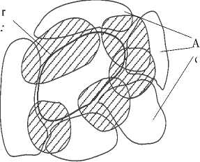
Delaunay triangulation [10, 42] is applied on P . The result is a set of triangular faces. By having Delaunay triangulation, no element of P will be inside the circumcircle of any triangle. The total length of Delaunay triangulation edges is minimal. Only the edges of the Delaunay triangulation are considered while finding the solution (i.e., while dividing the points into clusters). The algorithm for clustering consists of the following main steps: take one triangle from the center of the surface and consider its points as a first fragment of the first cluster; create the new cluster around the current fragment by adding new triangles in every next front (step) of the equal wave propagation from the current fragment by triangles in Delaunay triangulation that are adjacent to the triangles of previous front or by successively adding new triangles having the smallest area in each step; stop building the current cluster if the number of points in it is “close” to the maximum number n 0max ; take one of the adjacent triangles of the already created clusters and consider it as the first fragment of new cluster and create if there are more free triangles available; recursively repeat this operation; end the clustering process if there are no more free triangles available; search for all small clusters that have less than n_0min points, merge such two adjacent clusters together, or with a neighboring smallest cluster even if the merged cluster has more than n 0max points.

In Fig. 1, the set P has 160,000 points, the number of clusters is 156, the number of clusters after merging the smallest clusters is 135, approximate number of points in each cluster is 1000, and the lowest number of points in a cluster is 800.

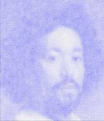
Pareja160K (TSP Art [24]) is shown in Fig. 1(a). Its decomposition by using equal wave propagation from the current fragment is shown in Fig. 1(b). The result by successively adding new triangles (having the smallest area) in every step is shown in Fig. 1(c).

• C.    Finding and merging the partial solutions

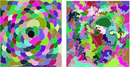
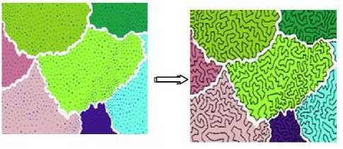
In the second stage, separate TSP solutions are found for each cluster. These solutions are merged together in the third stage to create an initial solution M_o for the whole problem. Fig. 2 contains the partial TSP solutions for some pieces of the Vangogh test-case. In the second stage, each partial solution can be found in parallel, as the calculations for finding the partial solutions are independent of each other.

The ring method [7, 8] is used to merge the partial solutions into one complete initial solution M_o . The process consists of the following steps (Fig. 3):

• 1.    Build an initial ring: Randomly select a cluster. The border of this cluster is created by the points that belong to the border triangles’ edges of this cluster (see Fig. 4). Every border edge has two incident triangles, one is internal and the other one is external to the cluster. The points of these triangles create an initial ring. These triangles are considered as the first front (step) for wave propagation. Every next front of wave propagation is performed by adding new points, from the adjacent triangles, to the current ring’s fragment.

  

  (b)

  (c)

  Fig.1. Pareja160K (TSP Art [23]) is in (a). Decomposition by using equal wave propagation from the current fragment is shown in (b). Successive addition of new triangles is shown in (c).

  
  

  2. Build the full ring: It consists of all the points that are obtained by wave propagation from the initial ring to a given number rin of internal triangles and a given number rout of external triangles. If the number rin is large enough, the final ring covers the entire cluster. The number of steps that needs to be performed for wave propagation is a parameter of the algorithm and this parameter depends on the number of points that must belong (approximately) to the ring. The ring creates overlapping zone that consists some points of the cluster that is currently considered (could be full but not necessarily) and some points of all the adjacent clusters. The number of wave propagation steps that needs to be performed in the internal and external cluster zones of the ring could be different.

  
  

• 3.    Replace all the pieces of routes that belong to the ring’s outside zones (external and internal) by temporary, fixed, and single edges having zero length. Let us call these temporary, fixed, and single edges as “temporary route segments”.

• 4.    Solve the TSP in the ring, by considering all its points in the ring and the temporary route segments (formed in Step 3) by applying the chosen TSP algorithm.

• 5.    Replace the temporary route segments by the real route pieces that have been removed in Step 3.

• 6.    Repeat all the previous steps for all other clusters that are not yet considered.

(a)

(b)

Fig.2. Pieces of Vangogh test-case (Fig. a) and the partial solutions for these pieces (Fig. b).

Algorithm: Merging the partial solutions.

Input data: Set of partial solutions, ring’s internal depth r in , ring’s external depth r out , and base TSP algorithm.

Output: Complete initial solution M 0 .

For each cluster

• 1.    Create the internal area of the ring using wave propagation, from the cluster’s border, on r in triangles.

• 2.    Create the external area of the ring using wave propagation, from the cluster’s border, on r out triangles.

• 3.    Replace all the rout segments, which are outside of the ring, by temporary segments.

• 4.    Find a solution for the ring using a base TSP algorithm by considering the temporary route segments.

• 5.    Replace the temporary route segments by the real route pieces and produce a complete initial solution M0.

Fig.3. Algorithm for merging partial solutions.

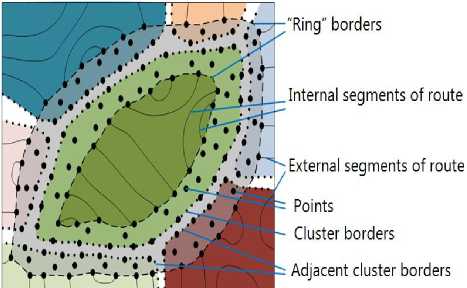
Fig.4. Clusters merging zone – “Ring”.

For parallel implementation, in Step 1, all the clusters whose rings do not overlap with each other will be considered simultaneously. The number of such steps is more than 4 as the chromatic number of a planar graph is 4. As a result, we receive one complete initial solution M₀ that passes through all the points of P .

• D. Optimization of the solution

The initial solution M 0 requires further optimization. It can be achieved by reducing the length of the route in the local optimization areas (LOA). The LOA consists of a small number of nearest points where there is a possibility of finding a better TSP (i.e., revising M₀ ). The LOA could be in the form of a circle, rectangle, or another kind of area. If better pieces of the route are found in the LOA then the existing segments of the route are replaced by the corresponding better ones.

To improve the initial solution, M₀ , the entire surface (all points of set P ) should be covered by such LOAs and the adjacent LOAs must overlap with each other. The quality of the final solution depends on the following parameters of the algorithm: the size (number of points) n sa in the LOA and the size of the overlapping areas n oa between LOAs. Increasing these sizes will improve the quality of the solution but it will increase the runtime. Some tradeoff must be made between these sizes. We proposed several methods to cover the entire surface by LOAs to improve the quality of the initial solution:

• 1.    SCB - by scanning along the cluster’s border with LOAs (Fig. 5). The centers c_i and c_i+1 of the LOAs are at the cluster’s border points. The points in the LOA are determined by wave propagation around its center with triangles. The border areas of all clusters must be considered.

• 2.    SR - by scanning along the route (i.e., overall solution) for LOAs (Fig. 6). The centers c_i and c_i+1 of LOAs are on the points of the route. The points in a LOA are determined by wave propagation around its center.

• 3.    SGA - by scanning over the whole surface by given geometrical LOAs such as rectangles (Fig. 7) or other. All the points of every LOA are considered. Some scanning strategy (i.e., the order of sequential steps), for example, horizontal, vertical, zigzag, or spiral, is chosen for this purpose.

• 4.    SCZ - by considering the specific critical zones that consist of a given number of neighboring points of three or more nearest (adjacent) initially created clusters (Fig. 8).

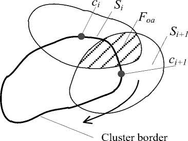
Fig.5. Scanning by LOA along the cluster border (SCB) – one step.

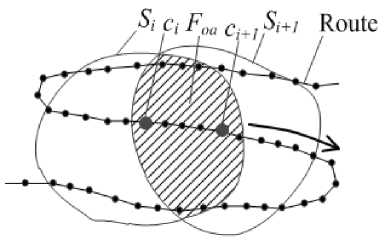
Fig.6. Scanning by LOA along the route (SR) – one step.

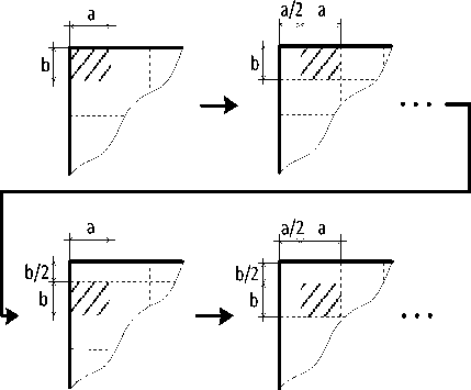
Fig.7. Scanning by rectangle LOA (a x b, shaded) over the whole surface (SGA) with shifting for every next sequential step in a/2 in horizontal and b/2 in vertical with 50% of overlapping.

Cluster border

djacent clusters

Fig.8. Optimization areas (shaded) for specific critical zones (SCZ).

For the first three strategies, optimization is performed by scanning the entire surface with LOAs. The parameters for these strategies are:

• 1.    Size, n_sa , of LOA (i.e. the number of points).

• 2.    Size, n_oa , of the overlapping area F_sa (i.e., the number of common points or the % of cluster’s points that are common) between adjacent S_i and S i+1 LOAs used by the sequential steps of the scanning process. In addition, the distance (i.e., number of points in the route) between the centers of the considered neighboring LOAs can be used, specifically for SCB and SR methods.

• 3.    Basic algorithm, for example LKH [16].

Based on the experimental results obtained, it is appropriate to choose n_sa between 800-1200 points, in order to obtain high quality solutions with a reasonable runtime. Experimental results show that if n oa is within 30-50% range of n_sa then we get good quality results.

Parallel algorithms can be used to optimize a few different non-adjacent LOAs whose full scanning areas do not overlap with each other. The new solution is accepted for the given area if the route’s length is less than that of the existing solution. The number of subsets of clusters a planar graph that can be considered independently (i.e., to apply the optimization on LOAs in parallel) is not less than 4 – the chromatic number of the planar graph whose vertices represent the clusters and the edges join such vertices whose full scanning areas overlap each other. For all clusters in each subset, the TSP can be performed simultaneously.

The experimental results show that the quality of optimization increases with the extension of the scanning and overlapping areas. However it increases the runtime. An optimal trade-off has to be found. It is suggested to repeat the scanning by changing the parameters and the scanning order (for example, scan in anti-clockwise direction rather than clockwise). Experimental results also show that an improvement is achieved through no more than 3-4 full cycles of optimization by using the same scanning parameters.

Specific critical surface zones (Fig. 8) include 3 or more adjacent clusters. These zones require additional improvements. For optimization in such zones, we use enlarged LOAs with 1200-1500 points or more.

Unfortunately, different optimization strategies cannot be executed in parallel because each optimization strategy requires the whole set of points P . However, some procedures in a single optimization strategy that don’t overlap with each other can be executed in parallel.

• IV.    Software for the Ring method

Parallel implementation requires efficient communications between the processors. In our experiments, Message Passing Interface was used for communications between the computer nodes. It allows scaling of TSP solver to a distributed system without major changes to the software architecture. The main stages of parallelization using different CPUs are shown in Fig. 9.

One CPU (CPU1) divides the given set of points into k different clusters. Each cluster is then assigned to a separate CPU. Partial TSP solutions are simultaneously produced from each of the clusters. These partial solutions are merged to form an initial and complete solution M₀ . A final optimized solution M f is developed from this solution. In the last stage, we use several optimization algorithms to produce a good quality final solution M f .

• V.    Experimental results

  The developed parallel ring method was investigated in terms of the quality of the solution and runtime. The TSP test-cases were taken from [11, 24, 25]. Experiments were conducted on a distributed system that contains Intel Xeon E5640 @ 2.67 GHZ CPU processors.

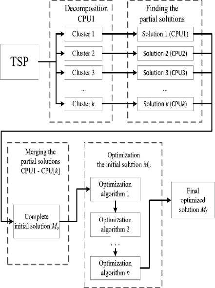
Fig.9. Main stages of Ring method.

The following parameters were used for merging the partial solutions:

• •    the number of points in cluster n_sa = 900;

• •    the internal depth of the ring r_in = 9 triangles (i.e.,

the ring covered 9 Delaunay triangles when propagating the wave from inside to the given cluster);

• •    the external depth of the ring r_out = 24 triangles

(i.e., the ring covered 24 Delaunay triangles when propagating the wave from outside to the given cluster).

The relations between different parameters of the clustering process, i.e., triangulation time t_t , number of points in clusters n₀ , runtime t_c , and the number of clusters k , are shown in Table 1. Triangulation time t_t takes approximately 10-15% of the entire decomposition process.

Table 2 shows the dependency of the sum of partial solutions, M Ʃps , on the size of the clusters (that are used for decomposition) for Mona-lisa test-case [21]. The table shows that an increment in the number of points in the clusters gives better results but it needs more runtime (the best-known length is 5757191).

Table 3 shows the comparison between the tour lengths before merging (sum of partial solutions M_Ʃps ) and after merging (the initial solution M₀ ) for some tests from TSP Art library [24]. The average quality improvement is approximately 1%. Better results (≈5%) were obtained for test usa115475 because we used larger inside and outside zones.

The dependencies between the duration, speedup, and efficiency (the ratio of speedup to the number of cores) of finding the partial solutions in parallel are shown in Fig. 10 (test E10M.0). The duration and efficiency are going down but speedup is increasing with the number of cores, but not proportionally, because the communication between the cores is increasing.

	Table 1. Dependencies in the decomposition process
Test-case	Number      Triangulation      Number       Runtime t c   Number of of points n         time (sec)       o po n s n 0        (sec)        clusters k in cluster
Mona-L. 100k Vang. 120k Venus 140k	100000           0.290          1000          1.505              96 2000          2.471              48 120000           0.357           1000          1.803             117 2000          2.961              58 140000           0.422           1000          2.094             137 2000          3.471              68
pareja 160k courbet 180k	160000           0.480           1000          2.387             157 2000          3.996              77 180000           0.541           1000          2.679             177 2000          4.454              88
earring 200k	200000           0.602           1000          2.960             198 2000          4.939              96
sra 104815	104815           0.198           1000          1.379             100 2000          2.351              51
ara 238025 lra 498378	238025           0.492           1000          3.131             232 2000          5.359             116 498378           1.090           1000          6.820            475 2000          11.51             238
E1M.0	106             3.799           1000           15.03              987 2000          24.80            493
E10M.0	107             74.41            1000           420.9            9906 2000          566.6           4961

Table 2. Dependency of Partial Solutions Sum M Ʃps from Cluster Sizes for Mona-Lisa Test Case [21]

n 0	k	t ps (sec)	M Ʃps
500	197	808	5856165
800	122	3104	5844204
1100	89	3560	5830572
1400	69	4408	5816598
1700	57	4144	5811076

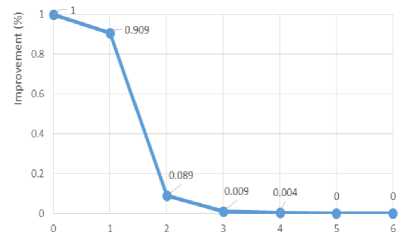
We tried to optimize the solution by scanning along the cluster border several times with the same values for the parameters. The experiment is aimed to find the number of iterations when further optimizations with the same parameters did not give further improvement. Fig. 11 shows the results with the test usa115475 [25] when 900 points were taken in LOAs with a distance of 54 points between them. As we can see, the fifth and further iterations did not give any further improvement in the quality of the solution. Therefore, to improve the quality of the solution further, the best way is to increase the size of LOA and decrease the distance between the LOAs (increasing the overlapping zone) and use different optimization algorithms.

Table 3. Comparison of Tour Lengths before and after Merging for Tests from TSP Art Library [24]

Test-case	M Ʃps (sum of partial solutions)	Number of points in cluster n 0	Inside depth r in	Outside depth r out	M 0 (initial solution)	% of reducing the ledge after merging
Mona-			3	6	5763878	0.9452
lisa	5818357	2500	6	6	5761695	0.9834
100K			9	6	5760264	1.0085
Vangogh 120K			3	6	6551963	1.1039
	6624291	1600	6	6	6549447	1.1428
			9	6	6548668	1.1548
Venus 140K			3	6	6819620	1.0261
	6889593	1600	6	6	6816208	1.0766
			9	6	6814392	1.1036
Pareja 160K			3	6	7630644	0.8962
	7699030	1600	6	6	7626749	0.9477
			9	6	7624413	0.9787
Courbet 180K			3	6	7902880	1.1013
	7989912	1600	6	6	7899127	1.1493
			9	6	7896762	1.1796
Earring 200K			3	6	8184591	0.8771
	8256382	1600	6	6	8180071	0.9329
			9	6	8177299	0.9671
			10	10	6216748	4.8755
Usa	6519843	2000	10	15	6213891	4.9237
115475			10	20	6210871	4.9747
			10	25	6209467	4.9984

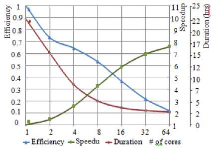
Fig.10. Dependencies between duration, speedup, efficiency, and number of cores for finding the partial solutions in parallel for test E10M.0.

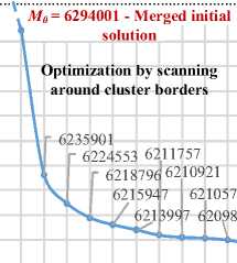
To improve the results, we investigated the possibility of sequential use of several optimization algorithms. Optimization by scanning around the cluster borders

(algorithm SCB, 9 steps 1-9) was performed during the first phase by taking the merged solution M₀ = 6294001 as an initial solution (Fig. 12 and Table 4). Specific critical zones (algorithm SCZ, 8 steps 10-17) were considered for the second phase.

# of iterations

Fig.11. Optimization process with the same parameters for the test usa115475.

Table 4. Two phases of sequential optimization on test-case usa115475

# of step	n oa	n oa		Length        I	Total mprovement improvement (%)               (%)		Runtime (min)	Total runtime (min)
PHASE 1. Sequential optimization by the scanning along the cluster border
0					M 0 = 6294001
	1	700	38	6235901	0.932	0.932	19	19
	2	725	40	6224553	0.182	1.116	18	37
	3	750	42	6218796	0.093	1.209	17	54
	4	775	44	6215947	0.046	1.256	14	68
	5	800	46	6213997	0.031	1.287	16	84
	6	825	48	6211757	0.036	1.324	17	101
	7	850	50	6210921	0.013	1.338	17	118
	8	875	52	6210578	0.006	1.343	18	136
	9	900	54	6209838	0.012	1.355	20	156
PHASE 2. Continuation of sequential optimization by considering the critical zones
	10	925		6208202	0.026	0.026	42	198
	11	950		6207820	0.006	0.033	44	242
	12	975		6207647	0.003	0.035	43	285
	13	1000		6207549	0.002	0.037	46	331
	14	1025		6207514	0.001	0.037	48	379
	15	1050		6207500	0.000002	0.038	50	429
	16	1075		6207484	0.000003	0.038	52	481
	17	1100		6207446	0.001	0.039	50	531

The experiment shows that it is useful to change the optimization algorithms to improve the quality of the solution. For the first phase, we received 1.4% improvement; and for the second phase, a 0.0001% improvement. Intel Xeon CPU E5-2620 v2 2.10GHz processor was used and parallel calculations were not used in this experiment.

ring covered 10 Delaunay triangles while propagating the wave inside the given cluster). External depth of a ring is r out =15 triangles (i.e., the ring covered 15 Delaunay triangles while propagating the wave outside the given cluster).

M Ʃps = 6716306 – Sum of partial \

Optimization for specific critical zones

6207820   6207500

6207647   ^6207484

0  1  2  3  4  5  6  7  8  9  10 11 12 13 14 15 16 17

# of iterations

Fig.12. Optimi z ation process with two algorithms for the test usa115475.

A significant feature of the developed approach is its near linear computational complexity (Table 5 and Fig. 13). Table 5 shows the dependency between the size of the problem, runtime, and the quality without parallelization. Experiments were conducted on a PC with Athlon II X2 240 processor with 2.8 GHz CPU and 2 GB RAM. The following parameters were used:

• •    The number of points in a cluster n sa = 800 to 900 and the size of the overlapping area n oa = 400.

• •    Internal depth of a ring r in = 10 triangles (i.e., the

Table 5. Experimental results for TSP Art library tests

Test with size	Length of the initial solution	Length of optimized solution	Run time (min)	Length of the best solution	Tour qualit y (%)
Mona-L. 100K	5758988	5757516	121	5757191	0.006
vangogh120K	6545620	6544127	178	6543622	0.008
venus140K	6812666	6811271	213	6810696	0.008
pareja160K	7622498	7620636	229	7619976	0.008
courbet180K	7891519	7889462	280	7888759	0.009
earring 200K	8174726	8174507	295	8171712	0.034

The results shown in Fig. 13 demonstrate that the developed approach is suitable for large-scale TSP problems to get high quality solutions in a reasonable amount of time.

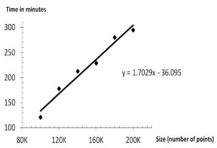
Fig.13. Time vs. size for TSP Art tests.

• VI. Conclusions

  • 1.    The developed approach for parallelization has near linear computational complexity and is suitable for large-scale TSPs.

  • 2.    The developed methods provide a significant reduction in runtime with a slight decrease in the quality of the received solutions, when compared with the other best known methods.

  • 3.    Higher speedup is achieved by using the problem decomposition to split the problem into several independent sub-problems that are solved in parallel.

  • 4.    Several optimization algorithms have been developed and investigated. To improve the quality of the solution, it is useful to successively apply different optimization algorithms.

  • 5.    The biggest problem solved by the developed implementation contains 10⁷ points. It needed 13 days time for calculations when a single CPU (Intel Xeon E5640 2.67GHz) was used. However, the same problem was solved in 28 hours by using cluster computing resources that contain 64 cores. In either case, the loss of the quality of the solution is very small (0.086% below when compared to the other best known solutions).

Acknowledgment

We thank the directors of the V.M. Glushkov Institute of Cybernetics of the National Academy of Science of Ukraine and the Institute for Condensed Matter Physics of Ukraine for providing cluster computing resources to perform our experiments. The work was performed in collaboration with the Vienna University of Technology and supported by the State Agency on Science, Innovations and Information of Ukraine.