A key assumption of the basic EOQ model is that stockouts are not permitted. Assuming that the lead time and demand are known and constant, this means that an order will be placed when the inventory available is exactly sufficient to cover the demand during that lead time. Under conditions of demand certainty, however, it is possible to prove that, assuming customers are always willing, although not necessarily happy, to wait for delivery, planned backorders can make economic sense, even if they incur some actual or implied cost. Relaxing the basic EOQ that stockouts are not permitted led to the development of EOQ model for the two basic stockout cases: backorders and lost sales. What took longer to develop was a model that recognized that, while some customers are willing to wait for delivery, others are not. Either these customers will cancel their orders or the supplier will have to fill them within the normal delivery time by using more expensive supply methods.

While there have been a number of models developed for the EOQ model with partial backordering, most of them incorporate considerably more complicated assumption sets than the classic EOQ model do. Therefore the objective of this paper is to develop a partial backlogging inventory model, and proposes a new algorithm to minimize the total cost, and finds the possible research direction of inventory control problems in the future.

• II.    Literature Review

Relaxation of the basic assumption that stockouts are not permitted led to the development of EOQ models for the two basic cases that occur when inventory is stocked out: backorders and lost sales. What took longer to develop was a model that recognized that, while some customers are willing to wait for delivery, others are not. This is commonly known as the deterministic EOQ model with partial backordering. A common characteristic of this model is the assumption that the percentage of orders arriving during the stockout period that will be backordered is exogenously determined. Montgomery et al.[4],Rosenberg[5],Park[6],San Joséet al.[7,8]and Pentico and Drake[9]all developed EOQ models with a constant backordering percentage. Montgomery et al. and San Joséet al. also developed models in which the backordering percentage depends on the time to replenishment. Chang and Dye[10])have considered inventory decisions for perishable items under partial backordering.

Deb and Chaudhuri[11] first proposed a allowed shortage inventory model by using heuristic method in 1987, where the demand function of the linear demand rate was considered. Mudueshwar[12] proposed the analysis procedure similar to Donaldson[13] to solve the optimal ordering time and frequency. Dave[14] amended the error in Deb and Chaudhuri model, including:

• (1)    The value of unit shortage cost per unit time;

• (2)    The total cost equation;

• (3)    The relationship between the number of shortage and order quantity, and proposed a reasonable Silver-Meal heuristic method.

Goyal, Morin and Nebebe[15] indicated that the total cost formula proposed by Deb, Chaudhuri and Murdeshwar are not correct, so he proposed correction method. Hariga[16] proposed a allowed shortage inventory model with the linear either increase or decrease demand rate by using numerical method. Abdel and Ziegler[17] considered a perishable product with constant demand, variable holding cost for different echelons, and proposed a two-echelon serial model without shortage. Reyes[18]presented an optimization model for a single period inventory problem in two-echelon supply chain. Lin and Lin[19]proposed a two-echelon inventory model for periodical goods that integrates the behavior of the manufacturer and retailers; and considered deteriorating items with completed backorder.

Due to the excess demands, stock-out situations may arise occasionally. Sometimes, shortages are permitted and they are backordered and satisfied in the very next replenishment. Hence, total inventory costs can be decreased substantially.

In some fashionable products, some customers would like to wait for backlogging during the shortage period. But the willingness is diminishing with the length of the waiting time for the next replenishment. The longer the waiting time is, the smaller the backlogging rate would be. The opportunity cost due to lost sales should be considered. Chang and Dye[20]developed an inventory model in which the demand rate is a time-continuous function and items deteriorate at a constant rate with partial backlogging rate which is the reciprocal of a linear function of the waiting time. Papachristos and Skouri[21]developed an EOQ inventory model with timedependent partial backlogging. They supposed the rate of backlogged demand increases exponentially with the waiting time for the next replenishment decreases. Teng et al. [22,23]then extended the backlogged demand to any decreasing function of the waiting time up to the next replenishment.

In this article, we developed a partial backlogging inventory model with stock-dependent demand rate, along with the effects of inflation and time value of money that are considered. We extended the model in Hou[24]to consider non-instantaneous and partial backlogging inventory model.

. . . , .        „ ,            s_n = 0 . .

• (4)    The initial time of shortage ⁰     , its inventory

level must be zero;

• (5)    Lead time is zero, and replenishment rate is infinity;

• (6)    There is no degradation in product;

• (7)    Shortage is allowed and happen in the beginning of any period;

• (8)    Consider the case of partial backlogging.

• IV.    Model Derived

Concerning the allowed shortage inventory model, we

, •             . .         .             . S n = 0

assume that inventory level must be zero when 0     , t. < s and the ordering behavior appears in time i i . Once ordering, products will be immediately sent. In addition, during the plan period, the shortage time in last shortage s„ = H\ period also meet accurately to the plan period ( n ).

The relationship between inventory levels and time is shown in Fig.1 in the allowed shortage inventory system. Q ( t )

s ₀

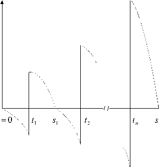
t n = H

Figure 1. the relationship between inventory levels and time

т h _t я ST (= [ Si- 1, ti ]) к 1 J

In any shortage period ⁱ i ¹ i ⁷, backorder

„ . . я .     11 + a(t, -1)     . s rate is defined as           i and

< t <  t i

,

i - 1

where a is expressed as backlogging parameter. Backorder rate means that the longer wait time (ti - t) , the fewer consumers will wait. Thus, in the i th shortage period, the time variable of the inventory level considering the partial backlogging can be expressed as dQi (u)         f (u)

du       1 + a ( t_i - u ) s i - 1 <  ^u <  ti

• III.    Model Assumptions

In ordering to simplify the problem, the reverse logistics inventory model must satisfy the following assumptions:

• (1)    Inventory system with the only species;

where

f ( t )

at time t

is expressed as instantaneous demand rate Since the boundary condition satisfies

• (2)    During the plan period

[0, H ]

permanently

Q ( S z 1) = 0

for i ¹⁷ in any period

, the purchase costs

are same and fixed, namely the cost is nothing to do with the order frequency and quantity;

• (3)    The demand rate is a known determinate strictly monotonic function;

i = 1 , 2 ,

....,n , the shortage quantity is defined by (1) as

SQ i ( u ) =

u        f ( t )

^s i - 1 1 + α ( t_i - t )

du

s

,

i - 1

≤ u ≤ t_i

Corresponds to the i th shortage period, the shortage cost can be defined as

SCi(si-1) =c3 ti    (ti-u) f (u)du si-1 1+α(ti -u)

where ( s_{i + 1}

t ^{i + 1 <  1 <}  s ^{i + 1} . According to Lemma 2 , period

-

t ^{i + 1} ) will be less than the previous period

(si -ti ) , so we get that   Qi(ti) will increase as i increases.

RT ( = [ t , s ] )

In ordering interval ^{i i i} , the holding cost

RC i ( t i )

is defined as

RC i ( t i )

si

= c    ( u - t ) f ( u ) du

² t i                ⁱ

c where 3 is expressed as unit shortage cost per unit time.

As this inventory model considers partial backlogging, therefore once shortage takes place, the loss cost of sale reduction is where c2

is expressed as unit the holding cost per unit time. Based on the above definition, the total cost can be described as

LC_i ( s_{i - 1} ) = c ₄ α ∫ ^ti ( t^{i -} u ) f ( u ) du ^{si - 1} 1 + α ( t_i - u )

n - 1 _s

W = nc ₁ + c ₂ ∑∫ ^{i + 1} ( u - t_{i + 1} ) f ( u ) du i = 0 ^{ti + 1}

c where 4 is expressed as the unit opportunity cost per unit time. And in i th ordering period, the time variable of the inventory level is

n - 1

+ ( c ₃ + α c ₄ ) ∑∫ i = 0

t i +1      ( t_{i + 1} - u )

^s i 1 + α ( t_{i + 1} - u )

V

f ( u ) du

dQ_i ( u ) _{- f ( )}

_du^u t _i ≤ u ≤ s _i

,

Since the boundary condition satisfies permanently

Q ( s ) = 0

for ⁱ in any period , , shortage quantity is defined by (5) as

....,

n , the

where c ¹ is expressed as the single ordering cost, n is the total ordering frequency.

Dealing with the allowed shortage inventory problem, the scholars often use the total cost of (9) divided by the

c holding cost per unit time 2 , so the above equation can be rewritten as

u

RQ i ( u ) = ∫ _tif ( t ) dt _{ti ≤ u ≤ si}

,

W = nM + ∑ ^{n - 1} ∫ ^{si + 1}( u - t_{i + 1} ) f ( u ) du i = 0 ^{ti + 1}

+(N +α O)∑n-1 ti+1 (ti+1-u)   f(u)du i=0 si 1+α(ti+1 -u)

Lemma 1 Suppose the demand rate f ( t ) is a strictly increasing function, period time will reduce with the ordering frequency i increasing, however the ordering RQ ( t )

quantity ^{i i} will increase as ordering frequency increases.

Prove We apply mean value theorem and assume that f ( t ) is a strictly increasing function, while the ordering quantity is

RQ i ( t i ) = ^si f ( u ) du = ( s i - t i ) f ( s i ) < ( s i +1 - t i +1 ) f ( θ 1 ) t_i

= ^{si +1} f ( u ) du = RQ i +1 ( t i +1 )

t i +1

W = ^W M = ^{c 1} N = ^{c 3} O = c ⁴

Where ^{c 2} 、 ^{c 2} , ^{c 2} , c ² .

• V.    The Necessary Condition of The Optimal Solution

st

We take (9) respectively to do ⁱ and ⁱ partial differential calculation, assuming under the condition of the given ordering frequency n , the necessary condition which minimizes the total cost must satisfy

∂ W                 t i         1

= ( c + c α )                   f ( u ) du

∂ t i      ^{34∫ s} i -1[ 1 + α ( t i - u ) ]²

• - c ₂ ^si ( u - t_i ) f ( u ) du

ti

• = 0, i = 1, 2,..., n

  д W ^д s i

  
  

  = ( c 3 + c ₄ a )

  
  

  ⁽ ti +i ^- s )

  ^{1 + a (}t i +i ^- s i )

  
  

  - c 2 ⁽ s i ^- t i )

  = 0, i = 1, 2,..., n

  
  
  
  

  Lemma 2

  
  

  Suppose the demand rate

  
  

  f ( t )

  is a strictly

  
  

  increasing function, period time will reduce with ordering frequency i increasing.

  
  

  Prove

  
  

  Suppose f ( t )

  
  

  is a strictly increasing function,

  
  

  VI . D ETERMINE O RDERING P ERIOD t ¹

  Appropriate ordering period t ¹ conduces to reduce calculation time, but past research has not proposed the determination mode of ordering period t ¹ for the partial backlogging problem. Therefore, this paper proposes the determination mode of the ordering period t ¹ for the partial backlogging inventory model. The paper tries to use the relative total cost minimization to derive the optimal ordering period t ¹ . First, the relative total cost is defined as

  
  

  we use mean value theorem to solve (11) and can get as follows

  
  

  ( c 3 + c ₄ a )

  
  

  ⁽ t i ^- s i - i )

  ¹ + ^{a (} t i ^- s i - i )

  
  

  TRCUT ( T ) = T

  
  

  T

  M + J ( u - t ₁ ) f ( u ) du

  
  

  \

  
  

  f ( 0 1 )

  
  

  + ( N + a O ) f t ‘ ⁽ t ¹ u ) f ( u ) du _v              ^{J 0} 1 + a ( 1 ₁ - u )          ₄

  
  

  = c 2 ⁽ s i ^- t i ) ^f ( ⁰ 2 )

  
  
  
  

  , s. . <  0 . <  ti    J ti <  d <  ^Si л *

  where i ^{1     1} i and i ² i . According to

  
  

  (12), we know

  
  

  ST (= [0. t . ])      . . .

  where shortage period is ¹       , ¹ , and ordering

  • . • RT ( = [ t. , T ])         _{f               л} ox _t .

  period is ^{1     1} ,      . Therefore we take (18) to do

  period time T differential calculation, to minimize the relative total cost period time must satisfy

  
  

  ( c ₃ + c ₄ a )

  
  

  ⁽ t i + 1 ^- s i )

  ^{1 + a (} t i + 1 ^- s i )

  
  

  = c 2 ⁽ s i ^- t i )

  
  
  
  

  dTRCUR (T ) = 0 dT ~

  
  
  
  

  Taking above formula into (13), we can obtain

  
  

  Expanding the above formula, we can get

  
  

  ⁽ t i ^- s i - 1 )

  ¹ + ^{a (} t i ^- s i - 1 )

  
  

  f ( 0 1 ) =

  
  

  ⁽ t i + 1 ^- s i )

  ^{1 + a (} ti + 1 ^- s i )

  
  

  f ( 0 2 )

  
  

  Since

  
  

  f ( t )

  
  

  is a strictly increasing function, then

  
  

  M + ( N + a O ) f t ¹    u f ( u ) du

  ^{J 0} 1 + a u

  T                           T

  +   ( u - T ) f ( u ) du = T  f ( u ) du

  t 1                                                                t 1

  
  
  
  

  f ( 0 1 ) <  f ( 0 2 )

  
  

  we can rewrite above formula as

  
  

  ⁽ t i ^- s i - 1 )     >     ⁽ t i + 1 ^- s i )

  ^{1 + a (} t i ^- s i - 1 )   ^{1 + a (} t i + 1 ^- s i )

  
  

  c       g ( u ) = 1/(1 + a u ) , _a > о

  Suppose                   ⁷, where ^a — ^v, and take

  it first-ordering differential

  
  

  dg ^{( u} ) = -—

  du (1 + a u )

  
  

  > 0

  
  
  
  

  For any increasing

  
  

  u >  0

  
  

  g ( u )

  
  

  is permanent a strictly

  
  

  function, therefore period time

  
  

  ⁽ ti ^- s i - 1 ) >  ⁽ t i + 1 ^- s i )

  
  

  , which proves that period time

  
  

  will reduce with the ordering frequency i increasing.

  
  

  VII. Algorithm

  The proposed algorithm in this section can be used in the linear demand rate, also in the nonlinear or transcendental function demand rate. The calculation process is as follows:

  • (1)    Make r = ⁰ , initial time s ⁰ ^ , plan time H , tolerate error ^to l = ¹⁰ , at the same time sets ordering time t ¹ and controls step size;

  • (2)    Rewrite ordering frequency as ^r ^ ^{r + 1} , and

  _t               г           n add = 0

  reset the added ordering frequency as _

  • (3)    Substituted into the equation ts

  (c3 + c4a)[ i f (u)/[1 + a(tt - u)]2 du = c2[ (u - tt) f (u)du s,-1

  *

  s .- ^ s

  to solve ⁱ ; then resubstituted into

  **

  ^{( c} 3 ^{+ c} 4 ^{a )(} t ^- s i VQ ^{+ a (} t ^- s i )) = ^c 2 ⁽ s i ^- t i )

  
  

  *

  to solve ^{i + 1}       . Furthermore we change ordering

  n add = n add + 1

  frequency _         _ to calculate shortage

  
  

  and ordering time sequentially. If

  
  

  (H - s ) > tol

  ⁿ , then

  
  

  TABLE I.      computational results

  total order number	total cost
  7	117.4409
  6	117.4323
  5	120.8574

  
  

  we adjust     t ₁ ′ = t ₁ + ( H - s_n )/step size until

  
  

  (H - s n ) ≤ tol

  
  

  to calculate the total cost W ;

  
  

  (4) To determine the direction of the total cost

  
  

  According to the numerical results in Table 2, shortage period and order cycle have shown a regular decrease and also prove Lemma 1. shortage interval is

  
  

  reducing and amend ordering time ¹ , return to step 2;

  (5) To calculate shortage, ordering time and the total cost sequentially.

  
  

  ST = t - s

  expressed as ^{i i     i - 1}

  
  

  RT = s - t

  expressed as ^{i i i}

  
  

  .

  
  

  holding interval is

  
  

  • VIII. Numerical Examples

  According to the above proposed method, this paper uses mathematical software MATLAB7.0 as the calculation and analysis tool. The example in this research derived from Donaldson[13], and add shortage cost, opportunity cost and backlogging parameter. The parameters are as follows:

  • (1)    non-linear increasing demand function ;

  • (2)    single ordering cost = 9;

  • (3)    unit holding cost per unit time = 2;

  • (4)    unit shortage cost per unit time = 7;

  • (5)    unit opportunity cost per unit time = 1;

  • (6)    backlogging parameter = 20;

  • (7)    plan period = 1.

  Based on the proposed method of the section, the total order number is 6 times which the minimum total cost is 117.4323.

  
  

  TABLE II.     O rdering time and cycle time

  Ordering Number i	Ordering time		cycle time
  	t i	si	ST i	RT i
  1	0.1245	0.3150	0.1245	0.1905
  2	0.3347	0.4860	0.0197	0.1513
  3	0.5004	0.6323	0.0144	0.1319
  4	0.6445	0.7642	0.0121	0.1197
  5	0.7749	0.8859	0.0108	0.1109
  6	0.8957	1.0000	0.0098	0.1043

  
  

  Since the inventory model adopts afterwards replenishment mode, therefore the ordering

  
  

  quantity

  
  

  RQ i '( = SQ i + RQ i )

  
  

  needs to replenish the

  
  

  shortage, in addition to purchase current inventory. The

  
  

  results in table3 also shows that quantity appears the regular increasing tendency.

  
  

TABLE III. calculation results of shortage and ordering quantity

Ordering Frequency	shortage quantity	Ordering quantity	actual ordering quantity
i	SQ i ( t )	RQ i ( t )	RQ i ( t ) ′
1	4.2136	37.6777	41.8913
2	4.8551	55.8777	60.7328
3	5.6366	67.2469	72.8835
4	6.2495	75.8515	82.1010
5	6.7588	82.9127	89.6715
6	7.1987	88.9717	96.1703

Sensitivity analysis can help us to observe the influence that the diversifications of inventory cost, demand and time affect the total cost. The paper analyze the parameters of this example, including H , c ¹ , c ² , c ³ , c ⁴ . The sensitivity of optimal ordering frequency is defined as follows.

*

S_n = ^{n n} × 100 % ⁿ                                         ( 21 )

While the sensitivity of the optimal total cost is defined as follows.

SW

W ^* - W

W

× 100 %

（22） where n and W respectively expresses the total ordering frequency and the minimum total cost the after parameters being changed.

The results of sensitivity analysis indicate that the plan period H is more sensitive parameter in all parameters; Otherwise, backlogging parameter α , cc shortage cost 3 and the opportunity cost 4 are less sensitive. In addition to ordering costs, the order number of all parameters increased with the parameter.

table iv.   Sensitivity analysis

Parameter	Change Rate	Order Number * n	Minimum total cost W *	n (%)	S W (%)
H	+50%	12	214.2290	100.00%	82.43%
	0%	6	117.4323
	-50%	2	42.0303	-66.67%	-64.21%
c 1	+50%	5	143.3575	-16.67%	22.08%
	0%	6	117.4323
	-50%	9	82.8446	50.00%	-29.45%
c 2	+50%	8	139.3573	33.33%	18.67%
	0%	6	117.4323
	-50%	5	86.0051	-16.67%	-26.76%
c 3	+50%	7	118.2377	16.67%	0.69%
	0%	6	117.4323
	-50%	6	116.1250	0.00%	-1.11%
c 4	+50%	7	119.3310	16.67%	1.62%
	0%	6	117.4323
	-50%	6	112.3916	0.00%	-4.29%
b	+50%	8	143.4732	33.33%	22.18%
	0%	6	117.4323
	-50%	4	83.0195	-33.33%	-29.30%

As this paper focuses on partial backlogging inventory model, so we specifically discussed backorder parameters., we can conclude the following from Table 5:

• (1)    With the increase in backorder parameter, the total cost and ordering number will also increase;

• (2)    When backorder parameter approaches zero, the total cost will be close to completely backorder model;

• (3)    When backorder parameter approaches infinity, the total cost will be close to not allowed out of stock model.

TABLE V. sensitivity analysis of backorder parameter

completely backorder	. . ,                           ГУ b acklogging parameter				not allowed backorder
	10	20	30	50
106.8811	114.5741	117.4323	118.7454	120.1319	125.2604

• IX. Conclusions

The purpose of this study is to simulate more reasonable market competition condition, and relax the previous research assumptions. The partial backlogging inventory model proposed in this paper makes the inventory model more reasonable during shortage period, at the same time also propose the prediction method and algorithm of ordering period t ¹ . Finally, the paper proposes a practical example of the numerical analysis. The inventory model proposed in this paper can provide the reverse logistics enterprise a appropriate assessment method dealing with the shortage problem, so they can work out a more reasonable inventory strategy.

Acknowledgment

The authors sincerely acknowledge the anonymous referees for their constructive suggestion.