A Performance Evaluation of Improved IPv6 Routing Protocol for Wireless Sensor Networks

Author: Vu Chien Thang, Nguyen Van Tao
Journal: International Journal of Intelligent Systems and Applications(IJISA) @ijisa
Article in issue: 12 vol.8, 2016.
Free access
In the near future, IP-based wireless sensor networks will play a key role in several application scenarios such as smart grid, smart home, healthcare, and building automation... An IPv6 routing protocol is expected to provide internet connectivity to any IP-based sensor node. In this paper, we propose IRPL protocol for IP-based wireless sensor networks. IRPL protocol uses a combination of two routing metrics that are the link quality and the remaining energy state of the preferred parent to select the optimal path. In IRPL protocol, we combine two metrics based on an alpha weight. IRPL protocol is implemented in ContikiOS and evaluated by using simulation and testbed experiments. The results show that IRPL protocol has achieved better network lifetime, data delivery ratio and energy balance compared to the traditional solution of RPL protocol.
Improved IPv6 routing protocol, wireless sensor networks, contiki operating system, network performance evaluation
Short address: https://sciup.org/15010881
IDR: 15010881
Text of the scientific article A Performance Evaluation of Improved IPv6 Routing Protocol for Wireless Sensor Networks
Published Online December 2016 in MECS
Internet of Things (IoT) [1] is a scenario in which the billions of devices are connected together and each device has a unique global address. In this scenario, IPv6 Wireless Sensor Networks (WSNs) have a key role since they will be used to collect several environment information. The applications of WSNs such as healthcare, building automation, and smart grid,...[2] with multi-hop communication model that use IEEE 802.15.4 standard will also be a part of IoT [3].
At the beginning, the wireless sensor network community rejected the IP architecture based on the assumption that it would not meet the challenges of wireless sensor networks. In fact, many have moved to IP because of the interoperability with existing systems and the well-engineered architecture based on the end-to-end architecture.
Therefore, the Internet Engineering Task Force (IETF) has created 6LoWPAN (IPv6 over Low-Power Wireless
Personal Area Networks) and RoLL (Routing over Low-power and Lossy networks) working groups to standardize the IP architecture for WSNs [4]. While the work from the 6LoWPAN working group opened the possibility of using IPv6 in IEEE 802.15.4 networks, standardizing a routing protocol was outside the scope of that working group. This led to the creation of the RoLL working group in 2008. RoLL Working Group has studied on standardization issues of IPv6 routing protocol for constrained devices over low-power and lossy networks. This group has proposed RPL protocol as an IPv6 routing protocol for WSNs.
In [5], Nguyen Thanh Long et al. presented a comprehensive study of the performance of RPL when compared to collection tree protocol. The study shows that the number of switching parents (Churn) in the RPL network is very low. Currently, RPL uses ETX (expected transmission) as its routing metric to avoid lossy links [6]. However, ETX doesn’t address the problem of energy balancing. Therefore, RPL is prone to the hot spot problem: certain nodes belong the routes that have good link quality will carry much heavier transmission load than other nodes. These nodes are likely to run out of battery faster than the ordinary nodes, which may create holes and undermine the network lifetime. In this paper, we will propose improved RPL (IRPL) protocol in order to overcome this disadvantage of RPL protocol. IRPL uses two routing metrics that are ETX and the energy state of sensor nodes to choose the optimal path. The contribution of this paper is threefold: Firstly, we propose a combined routing metric and show how to estimate it for each node; Secondly, we present an algorithm to choose the optimal path based on this routing metric; Finally, we implement and evaluate our proposal by using simulation and testbed experiments.
The remainder of this paper is organized as follows. Section II shows the related works. Section III introduces IRPL’s implementation principle. In section IV, the performance of IRPL protocol is evaluated and compared to the original RPL protocol; Finally, we conclude the paper.
-
II. R ELATED W ORKS
Routing in WSNs has been extensively studied in the last decade. Since most of the sensor nodes are battery powered, then a good routing protocol should save energy. In this section, we will present the descriptions and the implementations of RPL. Then, we will present the related works specifically for energy efficiency at the routing layer in WSNs.
-
A. Descriptions of RPL
RPL is designed for WSNs where sensor nodes are interconnected by wireless and lossy links. The lossy nature of these links is not the only WSN characteristic that drove the design decisions of RPL. Because resources are scarce, the control traffic must be as tightly bounded as possible. In these networks, the data traffic is usually limited and the control traffic should be reduced whenever possible to save bandwidth and energy.
RPL is a distance vector protocol that builds and uses DODAG in the network to perform routing [4]. In which, a DODAG is a network topology where all links between nodes in the DODAG has specified direction, toward the DODAG root. Fig. 1 illustrates an RPL DODAG.
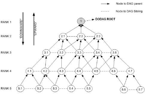
Fig.1. An RPL DODAG.
First, one or more nodes are configured as DODAG roots by the network administrator. RPL defines three new ICMPv6 messages called DODAG Information Object (DIO), DODAG Information Solicitation (DIS), and Destination Advertisement Object (DAO) messages. DIO messages are sent by nodes to advertise information about the DODAG, such as the DODAGID, the OF, DODAG rank, along with other DODAG parameters such as a set of path metrics and constraints. DIS messages are used to solicit DIO from an RPL node. A node may use DIS messages to probe its neighborhood for nearby DODAGs.
RPL uses “up” and “down” directions terminology. The up direction is from a leaf toward the DODAG root, whereas down refers to the opposite direction. The usual terminology of parents/children is used. RPL also introduces the “sibling”: two nodes are siblings if they have the same rank in the DODAG. The parent of a node in the DODAG is the immediate successor within the
DODAG in the up direction, whereas a DODAG sibling refers to a node at the same rank.
-
B. Implementations of RPL
Currently, several uIP stacks are available such as uIPv6 in ContikiOS; Blip in TinyOS [7]... These uIP stacks are lightweight and can be ported in several microcontrollers of sensor nodes including the MSP430 from Texas Instruments and the AVR ATMega128 from Atmel. Therefore, all the wireless sensor networks can be connected to the Internet as any computer devices.
The first draft of RPL was launched in August 2009 by IETF. One year later, the implementations of RPL were performed for TinyOS and ContikiOS. In [8], J. Tripathi et al. presented a performance evaluation of RPL. The authors use OMNET++ to simulate RPL. Some metrics for evaluation of RPL also are presented such as routing table size, expected transmission count, control packet overhead, and loss of connectivity.
At the same time, Nicolas Tsiftes et al. presented the first experimental results of RPL which they obtained with their ContikiRPL implementation [9]. They evaluate the power efficiency of ContikiRPL by running it in a 41-node simulation and in a small-scale 13-node Tmote Sky deployment in an office environment. Their results show several years of network lifetime with IPv6 routing on Tmote Sky motes. In [10], the authors presented a framework for simulation, experimentation, and evaluation of routing mechanisms for low-power IPv6 networking in Contiki. This framework provides a detailed simulation environment for low-power routing mechanisms and allows the system to be directly uploaded to a physical testbed for experimental measurements. In [7], JeongGil Ko et al. presented two interoperable implementations of RPL for TinyOS and ContikiOS. They demonstrate interoperability between two implementations.
Currently, RPL uses ETX as its routing metric to avoid lossy links. ETX is the inverse of the product of the forward delivery ratio, Df and the backward delivery ratio, Db, which takes into account link asymmetry.
ETX = 1 ( 1 )
Db refers to the packet reception ratio, while Df refers to the acknowledgment reception ratio. Routing protocols based on the ETX metric provide high-throughput routes on multi-hop wireless networks [11], since ETX minimizes the expected total number of packet transmissions required to successfully deliver a packet to the destination. This will result in a minimum energy path. However, by using the minimum energy path to route all the packets, the nodes on that path will quickly run out of energy. It will not improve the lifetime of the whole network and the resulted topology will not be energy balanced. In order to avoid this problem, we propose IRPL. This is done by having residual energy as a decision factor in the routing tables and this information is exchanged between the neighboring nodes.
-
C. Energy Aware Routing
Many energy-aware routing protocols have been proposed to minimize the energy consumption and to prolong the network lifetime. In [12], Kamgueu et al. proposed to use RPL with a residual energy metric. However, they do not consider the radio link quality. Oana Iova et al. [13] proposed the Expected LifeTime (ELT) routing metric to estimate the lifetime of bottlenecks. The authors take into account both the amount of traffic and the link reliability to estimate how much energy such a bottleneck consumes on average. RPL was used as the routing protocol in [14] where the forwarding load is weighted between the members of the parent list. The weighting is based on the members’ residual energy. The transmission range dynamically adjusted to maintain k parents. In [15], Rahul C. Shah et al. proposed Energy Aware Routing (EAR). EAR also maintains a set of good paths instead of a single optimal path. It introduces an energy metric which is determined by both the cost to deliver a packet and the residual power of the intermediate node. EAR requires a node to choose one path from those paths probabilistically. The probability assigned to each path is determined by the energy metric of the path. IRPL is different from EAR in several aspects. First, EAR’s routing decision is based on the residual energy of paths while IRPL’s is based on the residual energy indicator of individual nodes. From our perspective, EAR ignores the energy differences of sensor nodes on the same path. A path is abundant in residual energy does not mean all the nodes on the path is abundant in residual energy. Second, EAR’s energy cost metric is based on the assumption that the accurate residual energy and transmission cost of energy can be obtained by sensor nodes. However, this is not true for some sensor platforms. In IRPL, the residual energy is estimated by software and this mechanism can be easily added to existing sensor platforms. The detail of IRPL will be presented in section III.
-
III. I RPL P ROTOCOL
In this section, we will present the design goal and some challenges of IRPL design. Then, we will present our solution for implementation of IRPL.
-
A. Design Goal and Challenges
The main goal of IRPL design is to balance the energy of sensor nodes that belong to the routes having good link quality and increase the lifetime of sensor nodes. Some challenges of IRPL design are:
First, we need to determine the residual energy indicator of each sensor node. The mechanism to determine the energy indicator must be easily added to existing hardware and software designs, without any additional hardware cost.
Second, we need to propose an algorithm to choose the optimal path based on two routing metrics that are ETX and EI of forwarded nodes. The chosen route must have good link quality and avoid choosing sensor nodes that run out of energy.
-
B. Design Solution
The residual energy of a sensor node is defined by (2). In (2), E residual , E 0 , E consumption are respectively the residual energy, the initial energy and the energy consumption of the sensor node.
E , = Еп — Е residual 0 consumption
The total energy consumption of the sensor node is defined as [16]:
Econsumption = U ( I a t a + It + I t t t + I r t r + ^ Idt ci ) (3)
i
Where U is the supply voltage, I a is the consumption current of the microcontroller when running, t a is the time in which the microcontroller has been running, I l and t l are the consumption current and the time of microcontroller in low power mode, I t and t t are the consumption current and the time of the communication device in transmit mode, I r and t r are the consumption current and the time of communication device in receive mode, I ci and t ci are the consumption and the time of other components such as sensors and LEDs...
In this paper, we evaluate the performance of IRPL on TUmote (Thai Nguyen University mote). TUmote is a hardware platform for extremely low power, high data-rate sensor network applications. Fig. 2 shows the structure of TUmote.
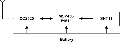
Fig.2. Structure of TUmote.
Table 1 shows our energy model, where the consumption currents are from chip manufacturer data sheets. In the energy model of TUmote, we only consider on the main energy consumptions that are the radio transceiver, the microcontroller, and the sensor, we ignore other small energy consumptions.
Table 1. Energy Model of TUmote
|
Component |
State |
Current |
|
MSP430 F1611 |
Active |
1,95 mA |
|
Low power mode |
0,0026 mA |
|
|
CC2420 |
Transmit (0 dBm) |
17,4 mA |
|
Listen |
19.7 mA |
|
|
SHT11 |
Active |
0,55 mA |
The energy indicator of the sensor node is defined by this equation:
EI (%) = E residuaL . 100% (4)
E 0
Fig. 3 shows the implementation of IRPL in Contiki operating system [17, 18]. We expand the routing table in ContikiRPL to store the information of residual energy indicator of neighbors. ContikiRPL uses ETX and EI metrics to choose the optimal path. The link estimator module will estimate the link quality. The energy estimator module will determine the residual energy indicator of the sensor node.
Algorithm 1: Preferred parent selection
Input: RoutingTable o/N
Output: preferred_parentofN best = NULL;
max_metricETx_Ei= ^ ^
for n = RoutingTablefi]
if (n.metricETx_Ei< max metric etx_ei) then max_metriCEix_Ei = n.metriCEixEii best = n;
end if end for if best ?= NULL then return best;
else send (DIS);
end if
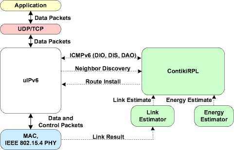
Fig.3. Implementation of IRPL in ContikiOS.
-
IV. P ERFORMANCE E VALUATION OF IRPL
-
A. Evaluation Metrics
We evaluate the performance of IRPL through a set of metrics that can outline the most significant features of the protocol.
Data delivery ratio: The first metric is the data delivery ratio (DDR). We define DDR as the ratio between the number of data packets received at the DODAG root and the number of data packets sent by nodes in the network.
In this paper, we propose a solution for combination of ETX and EI routing metrics by this equation:
metricETX £/(%) = a 100 + (1 - a )(100 - EI ) (5)
ETX _ EI ETX
Where α is the weight that allows adjusting between ETX and EI metrics in order to calculate the combined routing metric. The value of α weight ranges from 0 to 1; ETX max is the maximum value of route quality in the network. The combined routing metric is carried by the reserved field in DIO message. Fig. 4 shows the structure of DIO message [19].
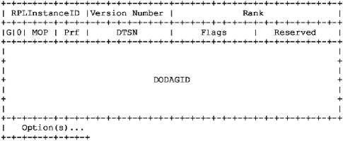
Fig.4. Structure of DIO message.
The goal of IRPL is to find the optimal path based on minimizing the combined routing metric. Algorithm 1 shows the pseudocode to select the preferred parent.
DDR (%) = N received- .100%
Ndata
In (6), N received is the number of data packets received at the DODAG root; N data is the number of data packets sent by all nodes in the network. Clearly, DDR equals to 1 indicates that the network can deliver all the data to the DODAG root.
Energy balance of routing protocol: We evaluate the energy balance of routing protocol based on the residual energy indicator. We calculate the energy balance indicator (EBI) as in (7).
N
EBI = \E ( EI - EI I )2
у i =1
In (7), EI reflects the average energy indicator of the whole sensor nodes.
Network lifetime: The main objective of any routing protocol is to extend the lifetime of WSNs. The network lifetime can be defined as the interval of time, starting with the first transmission in the wireless sensor networks and ending when the alive nodes ratio (ANR) falls below a specific threshold, which is set according to the type of application (it can be either 100% or less) [20].
ANR (%) = N alive nodes .W0% (8)
N
In (8), N alive_nodes is the number of alive nodes in the network; N is the total number of nodes in the network. If the threshold of ANR is set to 100%, then once the first node expires the network is considered expired as well.
-
B. Simulation and Evaluation
This section presents the performance evaluation of IRPL. We used the COOJA network simulator [18, 21] to simulate IRPL and analyze the results. In order to evaluate the benefits of IRPL for WSNs, we compared its performance to RPL’s. We evaluated the performance of two protocols with the same simulation scenario.
Fig. 5 shows the network topology of 26 nodes which are placed randomly in the sensor field and the node 1 is the DODAG root (Sink). The size of the network is 100m x 100m. Each node generates data packets for every 15 seconds. The sink collects the data packets and forwards the data packets to the PC.
Table 2 shows the simulation scenario in detail. We changed the alpha weight to evaluate the influence of this weight on the performance of the network. The value of α was chosen in the range of 0.8, 0.85, 0.9, 0.95.
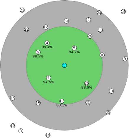
Fig.5. Network topology in the simulation.
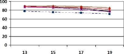
Fig. 6, 7, 8 show respectively the comparison between IRPL and RPL based on the alive node ratio, the data delivery ratio, and the energy balance indicator with different α.
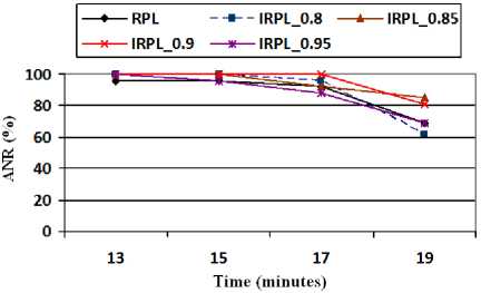
Fig.6. Comparison of alive node ratio in the simulation.
—♦—RPL --■--IRPL_0.8 * IRPL_0.85
—x—IRPL_0.9 ж IRPL_0.95
Time (minutes)
Fig.7. Comparison of data delivery ratio in the simulation.
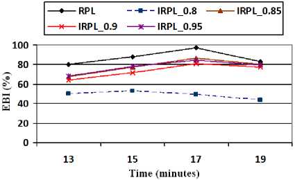
Fig.8. Comparison of energy balance indicator in the simulation.
Table 2. Simulation Scenario
|
Parameter |
Value |
|
Radio model |
UDI (Unit Disk Graph with Distance Interference) [22] |
|
Number of nodes |
26 |
|
Network size |
100m x 100m |
|
Communication range of node |
Transmission range: 30m, Interference range: 50m |
|
Initial energy |
10J |
|
Data packet interval |
15s |
|
Data packet initialization |
All nodes except the DODAG root |
|
MAC protocol |
CSMA/ContikiMAC [23] |
The simulation results show that IRPL with the α weight of 0.9 provides the best performance in terms of the alive node ratio (in Fig. 6). In this paper, we choose the threshold of ANR is 100% to determine the network lifetime. With this threshold, the network lifetime increases by up to 46% compared to the original RPL protocol. The simulation results in Fig. 7 also show that IRPL with the α weight of 0.9 achieves higher data delivery ratio than RPL does. From Fig. 6 and 7, we can see that IRPL with the α weight of 0.9 guarantees the best balance between the network lifetime and the data delivery ratio.
-
C. Testbed Experiments and Evaluation
IRPL is evaluated through a testbed (small-scale). The testbed results are used to calibrate the simulation results, and also to analyze the performance of IRPL in real experiments.
The experiments were carried out in the 1st floor of a smart home. The experiments consisted of 9 TUmotes in a grid topology and the sink on the edge, as depicted in Fig. 9. The experiments were carried out in an indoor environment. In this scenario, the nodes were deployed in rooms of the smart home. The experiments were conducted in a real world environment in the presence of continuous movement of people and other wireless network devices, which caused noise and interference.
Testbed experiments were also conducted to evaluate IRPL and compare its performance to RPL’s in terms of the network lifetime, the data delivery ratio, and the energy balance indicator in experiments into the real environment. The experiments were set up to allow each node to send a data packet to the sink with an interval of 30 seconds. In Fig. 9, the sink collects the data packets and forwards the data packets to the PC. From the simulation results, we chose IRPL with the α weight of 0.9. Table 3 shows the testbed scenario.
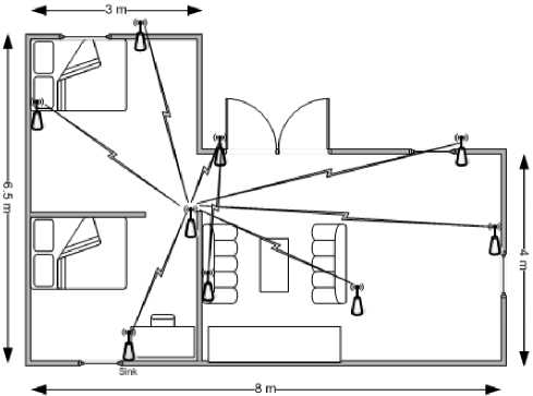
Fig.9. Network topology in the testbed.
energy consumption for all sensor nodes.
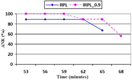
Fig.10. Comparison of alive node ratio in the testbed.
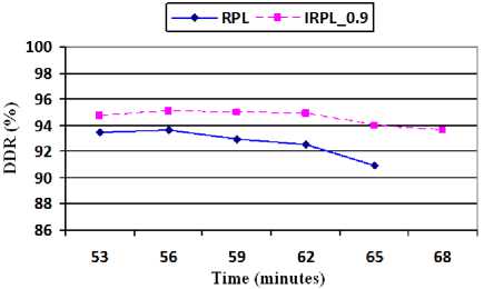
Fig.11. Comparison of data delivery ratio in the testbed.
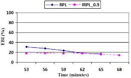
Fig.12. Comparison of energy balance indicator in the testbed.
Table 3. Testbed Scenario
|
Parameter |
Value |
|
Transmission environment |
Indoor |
|
Number of nodes |
9 |
|
Transmit power |
0 dBm |
|
Initial energy |
10J |
|
Data packet interval |
30s |
|
Data packet initialization |
All nodes except the sink |
|
MAC protocol |
CSMA/ContikiMAC [23] |
Fig. 11 shows the results of the data delivery ratio when using RPL or IRPL as the routing protocol. It is important to point out that IRPL achieves higher data delivery ratio than RPL does. This is due to the fact that the alive node ratio is higher when using IRPL. Thus, the more nodes survive in the network, the more data packets received at the sink.
Fig. 12 shows the energy balance indicator for this testbed. RPL presents unbalanced energy consumption between sensor nodes. IRPL does not increase energy consumption while improving the energy balance indicator.
Fig. 10, 11, 12 show respectively the comparison between IRPL and RPL for this testbed. The testbed results are also similar to the simulation results. Fig. 10 shows that IRPL increases the network lifetime by up to 17% compared to RPL. This is due to the fact that IRPL uses a load balancing scheme that provides uniform
-
V. C ONCLUSIONS
In this paper, we have proposed IRPL. IRPL uses two routing metrics that are the link quality and the residual energy indicator to select the optimal path. IRPL was evaluated by using simulation and testbed experiments to show its effects and benefits when compared to existing solution. Testbed results were used to calibrate and confirm the accuracy of the simulation experiments, as well as present the impact of IRPL in the real scenario. At the same time, the simulation experiments were useful to evaluate IRPL and compare it to RPL in terms of the alive node ratio, the data delivery ratio, and the energy balance indicator in the large-scale scenario. In the large-scale network, the simulation results showed that IRPL increases the network lifetime by up to 46% compared to RPL.
References A Performance Evaluation of Improved IPv6 Routing Protocol for Wireless Sensor Networks
- Luigi Atzori, Antonio Iera, Giacomo Morabito, “The Internet of Things: A survey,” Computer Networks, 54, pp. 2787-2805, June 2010.
- Hamida Qumber Ali, Sayeed Ghani, “A Comparative Analysis of Protocols for Integrating IP and Wireless Sensor Networks,” Journal of networks, Vol 11, No.1, January 2016.
- Md. Sakhawat Hossen, A. F. M. Sultanul Kabir, Razib Hayat Khan and Abdullah Azfar, “Interconnection between 802.15.4 Devices and IPv6: Implications and Existing Approaches,” IJCSI Int. Journal of Computer Science Issues, Vol. 7, Issue 1, January 2010.
- JeongGil Ko, Andreas Terzis, Stephen Dawson-Haggerty, David E. Culler, Jonathan W. Hui, Philip Levis, “Connecting Low-Power and Lossy Networks to the Internet,” IEEE Communications Magazine, pp. 96 – 101, April 2011.
- Nguyen Thanh Long, Niccolò De Caro, Walter Colitti, Abdellah Touhafi, Kris Steenhaut, “Comparative Performance Study of RPL in Wireless Sensor Networks,” in Proceedings of 19th IEEE Symposium on Communications and Vehicular Technology in the Benelux, 2012.
- JeongGil Ko, Joakim Eriksson, Nicolas Tsiftes, Stephen Dawson-Haggerty, Jean-Philippe Vasseur, Mathilde Durvy, Andreas Terzis, Adam Dunkels, and David Culler, “Beyond Interoperability - Pushing the Performance of Sensor Network IP Stacks,” in Proceedings of the 9th ACM Conference on Embedded Networked Sensor Systems (sensys'11), November 2011.
- JeongGil Ko, Joakim Eriksson, Nicolas Tsiftes, Stephen Dawson-Haggerty Andreas Terzis, Adam Dunkels and David Culler, “ContikiRPL and TinyRPL: Happy Together,” in Proceedings of the workshop on Extending the Internet to Low-power and Lossy Networks (IP+SN 2011), Chicago, IL, USA, April 2011.
- J. Tripathi, J. C. de Oliveira, J. P. Vasseur, “A Performance evaluation study of RPL: Routing protocol for low power and lossy networks”, in Proceedings of the 44th Annual Conference on Information Sciences and Systems, March 2010.
- N. Tsiftes, J. Eriksson, and A. Dunkels, “Low-Power Wireless IPv6 Routing with ContikiRPL,” in Proceedings of the International Conference on Information Processing in Sensor Networks (ACM/IEEE IPSN), Stockholm, Sweden, April 2010.
- N. Tsiftes, J. Eriksson, N. Finne, F. Österlind, J. Höglund, and A. Dunkels, “A Framework for Low-Power IPv6 Routing Simulation, Experimentation, and Evaluation,” in Proceedings of the conference on Applications, technologies, a rchitectures, and protocols for computer communications (ACM SIGCOMM), New Delhi, India, August 2010.
- De Couto D, Aguayo D, Bicket J, Morris R , “A high-throughput path metric for multi-hop wireless routing,” in Proceedings of the 9th Annual International Conference on Mobile Computing and Networking, New York, 2003.
- P. Kamgueu, E. Nataf, T. Ndié, O. Festor, “Energy-Based Routing Metric for RPL,” Research Report RR-8208, INRIA, 2013.
- O. Iova, Fabrice Theoleyre, and Thomas Noel, “Improving network lifetime with energy-balancing routing: Application to RPL,” in Proceedings of Wireless and Mobile Networking Conference, 2014.
- M. N. Moghadam, H. Taheri and M. Karrari, “Minimum cost load balanced multipath routing protocol for low power and lossy networks,” Wireless Networks, Volume 20, Issue 8, pp. 2469-2479, 2014.
- R. C. Shah and J. M. Rabaey, “Energy aware routing for low energy adhoc sensor networks,” in Proceedings of Wireless Communications and Networking Conference, 2002.
- Adam Dunkels, Fredrik Osterlind, Nicolas Tsiftes, Zhitao He, “Software-based Online Energy Estimation for Sensor Nodes,” in Proceedings of the 4th workshop on Embedded networked sensors, 2007.
- A. Dunkels, B. Grönvall, and T. Voigt, “Contiki – a lightweight and flexible operating system for tiny networked sensors,” in Proceedings of EmNets, pp. 455-462, 2004.
- J. J. P. C. Rodrigues and P. A. C. S. Neves, “A survey on IP-based wireless sensor network solutions,” Int. Journal of Communication Systems, Int. J. Comm Syst. 2010.
- Tsvetko Tsvetkov, “RPL: IPv6 Routing Protocol for Low Power and Lossy Networks,” Seminar SN SS2011 : Network Architectures and Services, pp. 59–66, July 2011.
- Roberto Verdone, Davide Dardari, Gianluca Mazzini, Andrea Conti, “Wireless Sensor and Actuator Networks: Technologies, Analysis and Design,” Academic Press, ISBN-10: 0123725399, 2008.
- Fredrik Österlind, Adam Dunkels, Joakim Eriksson, Niclas Finne, and Thiemo Voigt, “Cross-level sensor network simulation with cooja,” in Proceedings of the First IEEE International Workshop on Practical Issues in Building Sensor Network Applications (SenseApp 2006), Tampa, Florida, USA, pp. 641-648, November 2006.
- Azzedine Boukerche, “Algorithms and Protocols for Wireless Sensor Networks,” John Wiley & Sons Inc., ISBN: 9780470396360, 2008.
- A. Dunkels, “The ContikiMAC Radio Duty Cycling Protocol,” SICS technical report, December 2011.
