A Quality Assessment of Watermarked Color Image Based on Vision Masking

Digital watermarking is considered to be a most potential method of digital media copyright protection. Over the past decade, a lot of "Robust" watermarking systems were proposed[1-5]. With the continuous development of digital watermarking technology, performance evaluation research starts to receive people's attention[6-9]. Kutter and Petitcolas[6] pointed out that to evaluate the watermarking algorithm fairly, the fidelity of the watermarked image must be considered. Therefore, the quality assessment of the watermarked image is one of the most important aspects of the watermarking system performance evaluation. Quality assessment has been an important research subject in image processing and in digital watermarking field as well.

At present, there are two methods for the common quality evaluation of the watermarked image: subjective evaluation method and objective evaluation method. Subjective quality value is the most accuracy quality value. But the operation is complex, costly, and difficult to repeat. Therefore, ideally some automated mechanism for assigning a numerical value to the perceived quality of the watermarked image is desired. The commonly used objective evaluation method of watermarked image quality is the PSNR(peak signal-to-noise ratio). As we all known, PSNR is not so suitable to evaluate the image degradation introduced by the watermarking process. The results measured by PSNR do not match to human vision well.

There are some publications about the degradation evaluation of watermarked image. Bo, Shen and Chang[7] proposed a DCT(Discrete Cosine Transform) domain watermark assessment method based on Laplacian model. For the same watermarking algorithm, embed location and watermark sequence, the evaluation results become worse with the increase of the embed strength. The algorithm can’t distinguish the difference when we changed the length of embedded sequence under the same embed strength. By using the frequency masking, Ming, Hao and Yang[10] proposed a weighted image measurement, while the luminance and texture masking were not considered. By calculating the just noticeable difference (JND) for each DCT coefficient of image with watson’s JND model, Yang and Liang[11] assigned different weights for different components of image and achieved an optimized quality evaluation model. On this basis, Yang, Liang and others[12] added the color masking calculation and further improved the performance of the evaluation algorithm.

The organization of this paper is as follows. Section 2 analyzed the luminance, texture, frequency and color masking on human vision and given the calculation method of the four kinds of masking based on the psychophysical research and discrete cosine transform. In section 3, on the basis of the analysis above, we proposed a new quality assessment of watermarked color image, and noted it as MPSNR. Section 4 examined the performance of MPSNR. Section 5 given the conclusion inferred from this paper.

• II.    Calculation of visual masking

Embedding watermark will lead to the watermarked image quality decline in a certain extent. If it is considered as the result of noise that watermarked image quality reduced because of the embedded watermark, to assess the fidelity of the watermarked image, the original image noise masking ability should be calculated. Anderson and Netravali[13] proposed a noise visibility function. And the formula is:

NVF ( i , j ) =

.

У х M ( i , j ) + 1

Where У is a regulatory factor; M (i, j) is the noise shielding function. The variance of pixels in local area is usually treated as a function of noise shielding. Variance reflects the complexity of texture in image local area.

However, noise masking capability of image is not just the texture in image. According to psychophysical experiments, the image luminance of the background also plays a role in noise shielding.

• A.    Luminance masking calculation

  German experimental physiologist Weber discovered that the size of the difference threshold appeared to be lawfully related to initial stimulus magnitude in 1834. This relationship, known since as Weber's Law^[14], can be expressed as:

K-У

I

.

Where M represents the difference threshold, I represents the initial stimulus intensity and K signifies that the proportion on the left side of the equation remains constant despite variations of I . Therefore, the human eyes will have less sensitivity to modifications in high brightness area than in low brightness area, which is luminance masking.

Under normal illumination, the value of K is 0.02 in a wide range. Under the best illumination, the value of K is nearly 0.01. According to (2), for a given value of I , the just noticeable difference of brightness stimulus is:

У - KI .                 (3)

A lot of experimental results showed that it is the local area environment around pixel that affect the just noticeable difference, rather than the background environment of the whole image. The DC(Direct Current) coefficient of an 8 x 8 image block is the mean of luminance in 8 x 8 size of local area and can be used directly to calculate the image brightness intensity of the local area. Suppose X is a size of M x N gray image, and is divided into 8 x 8 non-overlapping sub-blocks. The pixel (i,j) in block (m,n) is noted as x _{i , j , m , n} . Each block is transformed into its DCT, and is written as y .

u , v , m , n

According to (3), we defined the luminance masking of the block (m,n) as:

y(0,0, m, n) ,, , m,n                                     .

y ( o , o )

Where y ( o , o , m , n ) is DC coefficient of block (m, n), m ∈ (0,1, ..., (M / 8 ) -1), n ∈ (0,1, ..., (N / 8) -1). y ( o , o ) is the mean of DC coefficients. Then we obtained a luminance masking matrix, ( L _{m , n} ).

• B.    Texture masking calculation

According to psychophysical experiments, the human eyes will have less sensitivity to modifications in texture area than in smooth area, which is texture masking.

To describe the texture situation in image, the gray-scale distribution of pixels and adjacent pixels need to be realized. AC(Alternate Current) coefficients reflect the pixels differences of the 8x8 local area in different directions at different scales. The background texture of 8x8 local area can be analyzed using the AC coefficients directly. We defined the texture intensity of sub-block (m, n) as:

^Tm , n    ^ m , n .                      ⁽⁵⁾

σ is standard deviation, the calculation formula is:

^ ² m , n - E {[ abs ( Y , n ) - E ( abs(Y_m n ))]²} . (6)

Where abs ( Y _{m , n} ) is an absolute calculation function. E ( abs ( Y _{m , n} )) is the expectation of abs ( Y _{m , n} ) . Y ( m , n ) is the AC coefficients. Combing (4) with (5), we defined a new noise masking function as:

M m , n - T m , n + L m , n .

Substituting (7) into (1), we obtained a new noise visual function:

NVF m,n

.

Ox M m , n + 1

θ is a regulatory factor.

In addition, according to psychophysical experimental research, the response of human visual cortex cells in their neighborhood show band-pass characteristics. The human eyes’ sensitivity to signals is different at different frequency channels. So, to evaluate image quality, the frequency masking on human vision should be considered, too.

• C.    Frequency masking calculation

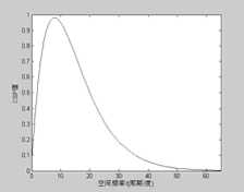
  F.W. Campbell published an article "space vision system through the information transmission" In 1974. He thought that vision system presents the characteristic of multi-channel^[15]. By using different spatial frequency raster images to test the sensitivity response of HVS (Human Visual System), the sensitivity curves of HVS for different frequencies can be obtained. Mannos, Sakrison and others set up the contrast sensitivity function (CSF) through a large number of experiments in [16]. The formula is:

A ( f ) - 2.6(0.0192 + 0.114 f )exp [- ( 0.114 f )'^J ]

Where f - ^f X + f y is spatial frequency (in cycles

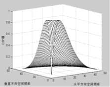
/ degree), f _x ， f _y is the horizontal, vertical direction of the spatial frequency, respectively. The corresponding spatial frequency characteristics curves of the function were shown in Fig.1.

(a)                           (b)

Figure 1. Spatial frequency curve of CSF

At the appropriate experimental conditions, a K x K size of image is transformed into its DCT, which is written as matrix y ( u , v ) ( u , v ∈ {0~ K -1}). The weighting coefficient of the DCT coefficient y ( u , v ) can be obtained by stretching the CSF to a K x K matrix. Table I showed a typical weighted coefficient matrix w ( u , v ) , which is corresponding to 8 x 8 transformation.

TABLE I.

The Weighted Matrix of DCT Coefficients by HVS Characteristics

0.4942	1.0000	0.7023	0.3814	0.1856	0.0849	0.0374	0.0160
1.0000	0.4549	0.3085	0.1706	0.0845	0.0392	0.0174	0.0075
0.7023	0.3085	0.2139	0.1244	0.0645	0.0311	0.0142	0.0063
0.3814	0.1706	0.1244	0.0771	0.0425	0.0215	0.0103	0.0047
0.1856	0.0845	0.0645	0.0425	0.0246	0.0133	0.0067	0.0032
0.0849	0.0392	0.0311	0.0215	0.0133	0.0075	0.0040	0.0020
0.0374	0.0174	0.0142	0.0103	0.0067	0.0040	0.0022	0.0011
0.0160	0.0075	0.0063	0.0047	0.0032	0.0020	0.0011	0.0006

From Table I we can see that the visual system is less sensitive in high frequency, and more sensitive in low frequency. The weighted matrix was written as w _{i , j} , and can be used to estimate the vision frequency masking. Using the weighted matrix w _{i , j} , we defined the formula of frequency masking as:

w f j =.                 (10)

^,     mean ( w _{i , j} )

mean ( w _{i , j} ) is the mean of w _{i , j} .

• D.    Color masking calculation

The matter may be much more complicated by different masking and pooling properties in the chromatic channels than in the luminance channel. To evaluate the degradation of watermarked color image, color masking should be taken into account. It is the same to the human color general knowledge that a true-color digital image can be described by R(red), G(green) and B(blue) matrices. A RGB image is an M x N x 3 array. Conventionally, the three M x N matrices may be called red, green and blue component, respectively.

The experiments indicated that the sensibility of human eyes to the change of red, green, blue is different, lowest to the change of blue color, highest to the change of green color. Except RGB color model, the NTSC color model is also commonly used, used in the television system in US. Main advantage of this system is that it is separate between gray information and the chromatic information, so the identical signal may be used in the chromatic TV set and monochrome set. In the NTSC model, the image is composed of three parts: luminance(Y), the tone(I) and the degree of saturation(Q). Luminance component indicates gray information, which is the collection of energy. Other two components express the chromatic information of the television signal. A formula is:

Y		0-299	0.587	0.114	R
I	=	0.596	- 0.274	- 0.322	G
Q		0.211	- 0.523	0.312	B

From the above formula, an equation is obtained, which is Y = 0.299 x R + 0.587 x G + 0.114 x B . The three coefficients in this equation reflect the different sensibilities of the human vision to the three color components of image. This characteristic can be used in image quality calculation. We estimated the color masking strength using this character and defined the calculation equation of the color image masking as:

C ( R , G , B ) = 3 x {0.299,0.587,0.114} (12)

Equation (8), (10) and (12) are the masking strength calculation formulas of color image masking on human vision and reflect the permission intensity of modification on different pixels. The bigger the masking strength is, the bigger the permission modification amount on the pixel is. With the same amount of modification, the bigger the masking strength is, the less the degradation of image quality is.

III.    MPSNR assessment of watermarked color

IMAGE

The commonly used objective evaluation method for a gray image is Peak Signal-to-Noise Ratio. The formula is:

PSNR = 10log10 M I N x ²⁵⁵ 2 .    (13)

УУ e ²( x , y )

xy

Where e(x, y) is the difference between the original image and the watermarked image. The size of the image is MxN. Corresponding to the color image, the PSNR may be expressed as:

PSNR = 10lg

3 x M x N x 255 2

У УУ e ²⁽ c , x , y )

c = R , G , B x y

Where c ∈ {R, G, B} indicates the color component. Equation (14) showed that the PSNR evaluates the image quality by calculating the whole difference between the original image and the watermarked image. So, firstly, PSNR can’t make a distinction between the big difference in local pixels and small difference in most pixels. Secondly, PSNR does not take in to account the brightness and texture masking on human eyes and can’t distinguish the difference between modification occurred in brightness and texture areas. At last, PSNR doesn’t consider the effect of different color masking on human vision. Therefore, PSNR evaluation result isn’t often consistent with the human visual sensation.

The masking of background luminance, texture, frequency and color on human vision in color images must be considered in image fidelity assessment. Similar to the conventional objective assessment PSNR, we used a logarithmic expression to calculate the quality of the distorted images. And the errors of different components between the original and the distorted images were weighted by (8), (10) and (12) that were presented above.

For a size of M x N x 3 original color image and its watermarked image X’, we calculated the error array between X and X’. The error array was divided into 8 x 8 non-overlapping blocks. Each block was transformed into its DCT, which was written as e _{i , j , m , n , c} . We weighted each DCT coefficient with (8), (10) and (12) as:

ev, j , m , n , c = ^{e x C (} c ) ^x e , j , m , n , c ^X f j ^{X NVF}m , n , c . ⁽¹⁵⁾

i,j ∈ {0,1,…,7}, m ∈ {0,1,…,(M/8)-1} ， n ∈ {0,1,…,(N/8)-1}, c ∈ {R, G, B}. β is a regulatory factor.

We calculated the inverse transform IDCT of e'    , i, j,m,n which was written as ew , and defined the watermarked i, j,c color image quality calculation formula as:

3 x M x N x 255 2 MPSNR = 10log10           w . (16)

A A ⁽ e j )

c = R , G , B i , j

Where i ∈ {0,1,…, M -1}, j ∈ {0,1,…, N -1}, c ∈ {R, G, B}.

Equation (16) is the new quality assessment of watermarked color image.

iv. Simulation and analysis

In this experiment, some watermarked images and other distorted images created by other distortion types were used to examine the performance of this new quality assessment. A watermarking algorithm was used to create the watermarked images. Some distorted images created by other distortion types were taken from LIVE (Laboratory for Image and Video Engineering)[17], which also offered the subjective quality values of these distorted images. We calculated the objective quality values of the distorted images using our quality assessment MPSNR, conventional assessment PSNR and other quality assessments proposed in [10], [11] and [12]. The correlation coefficients between the objective values and the different types of subjective values were calculated, and the performance of MPSNR was analyzed in the following.

• A.    The efect of assessing watermarked image quality

• 1)    Test one

The original images were shown in Fig.2. They are texture image “Baboon” and smooth image “Lena”. A spatial domain watermarking algorithm similar with that was proposed by Lu in [18] was used to create the watermarked color images. The watermark wi e {0,1} was composed of pseudo-random numbers, and obeys the Gaussian distribution. The locations where the watermark was embedded were pseudo-random positions within the B component of original color image. This position depended on a secret key, which was used as a seed to the pseudo-random number generator. The watermark was modulated and embedded into “lena” and “baboon” respectively using the methods presented by Lu. Strength factor a was changed from 0.01 to 2. Two groups of watermarked images of “lena” and “baboon” were obtained. Two objective assessments MPSNR and PSNR were used to calculate the quality of watermarked color image. The experimental results were presented in the following.

(a) lena

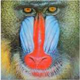
(b) baboon

Figure 2. Original images

(b)

(a)

Figure 3. The quality curves of the watermarked color images with the

watermark into B component.( a = 0.01~0.9)

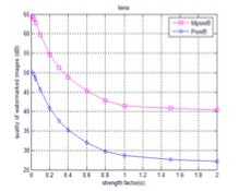
Fig.3 showed PSNR and MPSNR curves of the two groups of watermarked images of “lena” and “baboon”. X-coordinate is strength factor α and y-coordinate is the PSNR and MPSNR values, which is called quality decibel (dB). Usually, the larger the strength factor a is, the worse the quality of the watermarked image is at the same other conditions. From Fig.3 we can see that the MPSNR value decrease with the increase of strength factor a . This indicates that MPSNR can detect the strength of watermark. The MPSNR quality measurement is valid.

• 2)    Test two

According to section II.A in this paper, the human vision has different sensibilities to the change of different color. So, if the same watermark is embed into the different color components of the color image, the human eyes will have the different sensations.

Some particular watermarked images were created using a watermarking algorithm. The watermarking algorithm was similar to the one presented in test one. But the watermark was embedded into R and G components, respectively. Modulating the strength factor αfrom 0.01 to 2 and two groups of watermarked color images for original image “lena” were obtained, respectively. One group of image was R component watermarked color images. The other was G component watermarked color images. Together with the B component watermarked color images created in Test one, there are three groups of watermarked color images for each original color image. The experimental results were shown in Fig. 4 and Fig. 5.

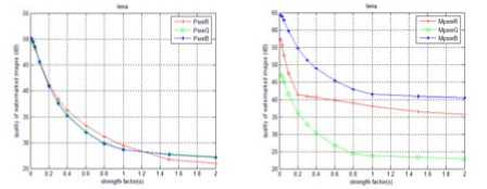
Three watermarked color images of “lena” and the corresponding quality values of PSNR and MPSNR were shown in Fig. 4. The embedding strength factor α was 1.5. Fig.4(a) showed a R component watermarked image of “lena”. Fig.3(b) showed a G component watermarked image of “lena”. Fig.3(c) showed a B component watermarked image of “lena”. In Fig. 5, the abscissa axis is the strength factor α , the ordinate axis is quality decibel (dB). Fig. 5 showed the curves of PSNR and MPSNR value with the factor α changed from 0.01 to 2. PsnrC and MpsnrC express PSNR and MPSNR quality decibel of C component watermarked image. C ∈ {R,G,B}) represents the color component.

(a)α=1.5,PSNR=26.733 (b)α=1.5,PSNR=27.724 (c)α=1.5,PSNR=27. 645

MPSNR = 36.499 MPSNR = 23.313 MPSNR = 40.791

Figure 4. Watermarked color images of “lena” when α =1.5, PSNR values and MPSNR values: (a)watermarked color image with watermark in R component; (b)watermarked color image with watermark in G component; (c)watermarked color image with watermark in B component

(a) PSNR quality curves

(b) MPSNR quality curves

Figure 5. The quality curves of watermarked color images: (a)The PSNR quality curves of lena’s three color component watermarked color images; (b)The MPSNR quality curves of lena’s three color component watermarked color images.

Firstly, we assessed the quality of images shown in Fig. 4 by human eyes. The result is: Fig. 4 (c) is the best; Fig. 4(a) is worse; Fig. 4 (b) is the worst.

Secondly, we calculated the quality values using PSNR. The result is: Fig.4(a) is 26.733; Fig.4(b) is 27.724; Fig.4(c) is 27.645. The three quality values extremely approach to one another, namely the three images have the same quality level according to PSNR. Obviously this is not consistent with the human visual sensation.

Finally, we calculated the quality vales using MPSNR. The result is: Fig.4(c) is 40.791, which is the best. Fig.4(a) is 36.499, which is worse. Fig.4(b) is 23.313, which is the worst. The quality of the three watermarked color images of “lena” judged by MPSNR is different obviously and is completely consistent with the human visual sensation.

Curves of Fig.5 expressed the similar conclusion above.

From above, it can be concluded that the quality evaluation method MPSNR proposed in this paper is obviously superior to PSNR. The result judged by MPSNR is more consistent with the human visual sensation than PSNR.

• B.    The efect of other distorted image quality assessing

LIVE provides samples of image. It also gives the subjective quality score DMOS. DMOS values rang from 0 to 100, the little number expresses the greater quality, the large number expresses worse quality. MPSNR, PSNR, the algorithms proposed in [10] (method10), the algorithms in [11] (method11), and the algorithms in [12] (method12) were used to calculate the quality of images in LIVE in this experiment. Following was the experimental results.

• 1)    Test one

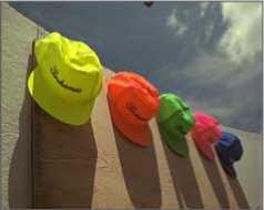
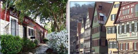
Some distorted images of a heavy texture image “building” and a smooth image “caps” are selected to examine the performance of MPSNR. Fig.6 showed four distorted images. They come from original heavy texture image "building" and smooth image "Caps". The subjective quality values DOMS and five objective quality assessment values of the four distorted images are illustrated in Table II.

(a)

(b)

(c)

(d)

Figure 6. The distorted images created by the same distortion type on different texture original images

TABLE II.

The Quality Values of Distorted Images in fig.6 According to Different Assessment

Method	Fig.6(a)	Fig.6(b)	Fig.6(c)	Fig.6(d)
DMOS	25.477	34.497	48.073	53.456
MPSNR	44.275	39.526	36.378	34.312
PSNR	29.307	35.81	21.207	30.073
Method10	35.57	41.654	27.1	34.865
Method11	21.461	31.167	18.7	26.432
Method12	25.669	26.961	13.794	21.482

From Fig.6 and the DMOS values shown in Table II we can see that the quality gradually decreases from Fig.6(a) to Fig.6(d). MPSNR showed the same result and is consistent with DMOS. PSNR values showed: Fig.6(b) is better than Fig.6(a) and Fig.6(d) is better than Fig.6(d). This is not consistent with DMOS. The other three methods give the similar result with PSNR. In this test, MPSNR outperforms the other four objective methods.

2)Test two

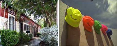
In this test, two different frequency texture images “building” and “buildings” are selected. Fig.7 showed four distorted images of the two texture images. The subjective quality values and the four kinds of objective method values are illustrated in Table III.

(a)                                   (b)

(c)

(d)

Figure 7. The distorted images created by the same distortion type on different trquence images

TABLE III.

The Quality Values of Distorted Images in fig. 7 According to Different Assessments

Method	a	b	c	d
DMOS	31.56	37.021	47.533	53.846
MPSNR	41.785	40.589	39.318	35.995
PSNR	26.088	28.989	24.189	24.601
Method10	32.645	35.171	30.41	30.238
Method11	22.725	25.47	21.057	21.671
method12	18.383	20.924	16.478	16.756

Fig.7 and the DMOS values shown in Table III showed that the quality values gradually decrease from Fig.7(a) to Fig.7(d). MPSNR is consistent with DMOS, showed the same result. PSNR values showed: Fig.7(b) is better than Fig.7(a) and Fig.7(d) is better than Fig.7(c). This is not consistent with the subjective values DMOS. The other three kinds of objective method give the similar results with PSNR. They are not consistent with DMOS. In this test, MPSNR outperforms the other objective methods.

From the last two tests we can see that the four kinds of objective method are worse than MPSNR in judging the fidelity of the different texture distorted images. They can't correctly judge the texture and frequency masking on human vision in image. So the conclusion can be drawn, that MPSNR outperforms the other four kinds of objective method. The MPSNR quality values are more consistent with the objective values DMOS than the other four objective assessments.

• 3)    The correlativity and consistency between the values of objective assessment and DMOS.

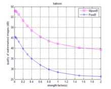
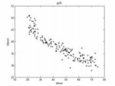
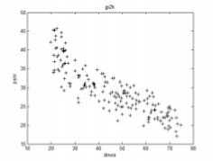
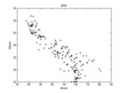
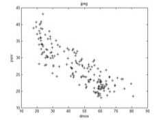
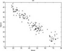
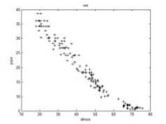
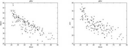
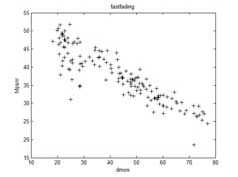
Further examine the performance of MPSNR, all distorted images in LIVE are assessing in the next experiment. There are five kinds of distorted images in LIVE: “Jpeg2000” distorted images, “Jpeg” distorted images, “White Gaussian noise” distorted images, “Gaussian Blur” distortion images and “Fast Fading Rayleigh” distorted images. The subjective-objective quality diagrams of the five kinds of distorted images were shown in Fig. 8 to Fig.12. Each diagram was titled with the distortion type. Abscissa is subjective quality values. Ordinate is objective quality values of MPSNR or PSNR.

(a)

(b)

Figure 8. “Jpeg2000” distorted images subjective-objective quality diagrams: (a) DMOS-MPSNR diagram; (b) DMOS-PSNR diagram.

(a)

(b)

Figure 9. “Jpeg” distorted images subjective-objective quality diagrams: (a) DMOS-MPSNR diagram; (b) DMOS-PSNR diagram.

(a)

(b)

Figure 10. “White Gaussian noise” distorted images subjective-objective quality diagrams: (a) DMOS-MPSNR diagram; (b) DMOS-PSNR diagram.

(a)                         (b)

(a)

Figure 12. “Fast Fading Rayleigh” distorted images subjective-objective quality diagrams: (a) DMOS-MPSNR diagram; (b) DMOS-PSNR diagram.

Figure 11. “Gaussian Blur” distorted images subjective-objective quality diagrams: (a) DMOS-MPSNR diagram; (b) DMOS-PSNR diagram.

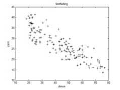
(b)

Fig.8 to Fig.12 showed that MPSNR-DMOS correlation is better than that of PSNR-DMOS. To give the accurate digit of the correlation between objective and subjective assessment, we calculated the correlation and consistency coefficients between objective quality values and DMOS by (17) and (18). Table IV and Table V illustrated the absolute values. The number approximate to 1 shows that the higher the correlation between the subjective quality and the objective quality.

corr ( x , y ) =

У x , y , i

1     .jyTTy

^T ( x, y ) =

P [( X i - Х у )( y,- - y j ) >  0 - p [( X i - x j )( У,- - y j ) <  0

TABLE IV

Correlation Coefficients Between DMOS and Objective E VALUATION R ESULTS ( corr )

Method	Distortion Types
	JPEG-2000	JPEG	White Noise	Gaussian Blur	Fast Fading Rayleigh
MPSNR	0.92526	0.89646	0.95173	0.82652	0.89283
PSNR	0.86675	0.85436	0.9778	0.77486	0.77486
Method10	0.88861	0.89474	0.98177	0.87362	0.88317
Method11	0.87474	0.88438	0.98139	0.8668	0.87332
Method12	0.87424	0.88053	0.98064	0.85362	0.88282

TABLE V

Consistency coefficients between DMOS and objective

EVALUATION RESULTS ( K ENDALL T )

Method	Distortion Types
	JPEG-2000	JPEG	White Noise	Gaussian Blur	Fast Fading Rayleigh
MPSNR	0.78825	0.69307	0.78697	0.65939	0.741
PSNR	0.69372	0.64355	0.8933	0.58621	0.70019
Method10	0.73021	0.68256	0.88736	0.72375	0.71877
Method11	0.71414	0.67113	0.8887	0.69368	0.70594
method 12	0.71372	0.66798	0.89195	0.6751	0.71935

In Table IV, the corr value of MPSNR for the “White Noise” images is the lowest in the 5 kinds of objective measurements. The corr value of MPSNR for the “Gaussian Blur” images is bigger than PSNR, and is lower than the other 3 kinds of objective measurements. Except “White Noise” and “Gaussian Blur” images, the corr values of MPSNR for the other 3 kinds of degraded images are all the maximum value in the 5 kinds of objective evaluation algorithm. So, we can draw the conclusion that the proposed algorithm in this paper outperforms the other 4 kinds of objective measurements, and has high correlativity with DMOS.

From Table V, we drew the same conclusion as mentioned above.

From the experimental results above, the conclusion can be drawn: the quality assessment proposed in this paper can represent the human perception well. The evaluation results have high relevancy and consistency with subjective evaluation, and present higher credibility.

V. Conclusions

Urgent social need promotes the development of digital watermarking technology. The performance evaluation of the watermarking algorithm has become a popular topic with the continuous development of digital watermarking. In this paper, we analyzed the image luminance, texture, frequency and color masking on human vision, and given a DCT coefficient noise masking function based on the psychophysical experimental research. On the basis of above, a new quality assessment of watermarked color image was proposed by weighting the different components of color image. Experimental results showed that the algorithm can correctly detect image degradation which is caused by watermarking process and other distortion types and have high relevancy and consistency with subjective values. The MPSNR quality values present higher credibility and can be used to evaluate the degradation of the watermarked image.

Acknowledgment

The author wishes to thank Dr. Haifeng He and Dr. Hua Zhao. This work was supported by the Encouragement Foundation for Excellent Young and Middle-aged Scientists of Shandong Province (Grant No. BS2010DX026); A Project of Shandong Province Higher Educational Science and Technology Program (Grant No. J10LG24); the Shandong Provincial Natural Science Foundation (Grant No.Y2008G11), China.