A Review of Methods of Instance-based Automatic Image Annotation

Author: Morad A. Derakhshan, Vafa B. Maihami
Journal: International Journal of Intelligent Systems and Applications(IJISA) @ijisa
Article in issue: 12 vol.8, 2016.
Free access
Today, to use automatic image annotation in order to fill the semantic gap between low level features of images and understanding their information in retrieving process has become popular. Since automatic image annotation is crucial in understanding digital images several methods have been proposed to automatically annotate an image. One of the most important of these methods is instance-based image annotation. As these methods are vastly used in this paper, the most important instance-based image annotation methods are analyzed. First of all the main parts of instance-based automatic image annotation are analyzed. Afterwards, the main methods of instance-based automatic image annotation are reviewed and compared based on various features. In the end the most important challenges and open-ended fields in instance-based image annotation are analyzed.
Automatic Image Annotation, Instance-Based Nearest Neighbor, Semantic Gap, Voting Algorithm
Short address: https://sciup.org/15010882
IDR: 15010882
Text of the scientific article A Review of Methods of Instance-based Automatic Image Annotation
Published Online December 2016 in MECS
Today, due to the increasing growth of digital images and the need to manage and retrieve them image annotation has become a dynamic field in research. The aim of annotation is to accompany the words denoting the meanings and concepts with the image. Interpreting this volume of images by human being is impossible, costly, and time consuming, so to automate the annotation process seems to be essential. However, information and features extracted from the images do not always reflect the Image content and the semantic gap as “the lack of coincidence between the information that one can extract from the visual data and the interpretation that the same data have for a user in a given situation” is known as the main challenge of automatic systems.
Recently, researches have focused on Semi-supervised systems so as to fill the semantic gap by helping data produced by users . Too many methods have been proposed in this field. Automatic Image annotation process is one of the applications of Machine Vision in image retrieving systems and it is used to organize and locate the existing images in sets. In text-based methods the retrieving process is based on texts and keywords written for each image. In this method whenever a query is received from a user the images enjoying that kind of query are retrieved.
Here in this paper the main parts of instance-based image automatic annotation are first analyzed.Afterwards, the main methods of instance-based automatic image annotation are reviewed and compared based on different features. The main existing challenges in this field are recognized and analyzed.
The rest of the paper is as follows: in the second part the main parts of instance-based automatic image annotation are briefly carried out, the most important and well-known algorithms of instance-based automatic image annotation are reviewed and compared with each other. And in the end the conclusion and open ended fields are proposed.
-
II. A R EVIEW OF THE M AIN P ARTS OF I NSTANCE -B ASED I MAGE A NNOTATION
The main parts of instance-based image annotation are shown in figure 1. In these systems the images of the data set are first read offline and the intended features of the images are extracted and a database containing feature Vectors are saved. In the next phase the image which is intended to be annotated is received from the input online as the query image. Again and identical to the offline phase, the intended features are extracted and there will be a vector of feature. In order to obtain intended tags from the existing images in the dataset the feature vector of the query image is compared with feature vectors of the images of the set for being similar by the help of Similarity measures to find the nearest image by the help of the nearest neighbor method. In the next phase the best tags are obtained for the query image by using methods such as voting the tags of the near images. Next, each part of instance-based automatic image annotation is analyzed separately.
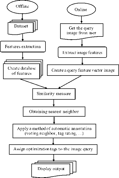
Fig.1. Schematics of annotations system
-
A. The images database
In instance-based automatic image annotation systems the images database plays a crucial role in precise automatic annotation. There various databases in this field that they each have different images and tags. Following this section the most important set of images which is used in various studies is analyzed:
-
• NUS-WIDE: This set has been prepared by Singapore National University and contains 269648 images. Of course this set is a set of images features vector with 501 dimensions. This set has become a reference set of images annotation. This set contains 81 tags.
-
• Mir Flickr: Mir Flickr database produced in Leiden University contains 25000 images and 38 tags and it is especially allocated for image retrieving enhancement. The images in Flickr have collected as metadata EXIF and they are readily available in text files.
-
• MIRFLICKR-25000: A big effort has been made to make an image set and evolving ideas. Image set prepare metadata and annotating. If one inserts one's email address before downloading, he/she can receive the latest updates.
-
• Corel5k: It contains 5000 images and 3 74 tags. However, Corel10k contains 10000 images in 100
groups. Every category contains 100 images of size 192×128 or 128×192 in JPEG format images. This set is only used for scientific communication not in commercial properties.
-
• IAPR TC12: This set contains 20000 images and 291 tags. TC-12 is used for evaluating image automatic annotation methods and studying their effects on multimedia information retrieving. The images are segmented and features are extracted from each segment and every single segment is tagged. Annotation is carried out in the region according to annotation hierarchy and spatial relationships information. Each image is manually segmented and the resultant regions have been annotated according to predefined words of tags.
-
• Wang: Exists 1000 color images in this data set which are organized in 10 groups. Each group contains images and textual description for a category of butterflies collected from Google through querying with their scientific names of the species, for instance "Danaus plexppus". They are also manually filtered for those depicting the butterfly of interest. The textual descriptions were obtained from the eNature online nature guide for every single butterfly.
-
• ImageNet: This set has been organized according to WordNet hierarchy. Each meaningful concept in WordNet, possibly described by multiple words or word phrases, is called a "synonym set" or "synset". There are more than 100,000 synsets in WordNet, majority of them are nouns (80,000+). Image Net aims at proposing average 1000 images in each synset to be shown. Each image is controlled for each high quality concept and annotated by human. ImageNet proposes millions of categorized images for many concepts in WordNet hierarchy.
-
• LabelMe: It contains 50000 JPEG images (40000 are used for training and the other 10000 for testing). The size of each image is 256 x 256 pixels. The performed annotation is in two different file formats. One of the amount of tags is between [-1.0,10]. 1.0 implies that the object in the image is similar to the extracted images. If no sample of the object class can be found in the image or different levels overlap each other, then the amount of the tag will be calculated as 1.0.
-
• Tiny Image: It contains images in size of 32 x 32 and they are created and saved as big binary files. 400Gb of free disk space is needed for this data set. This data set enjoys two versions of function for reading image data including: (i) Load tiny images.m - plain Matlab function (no MEX), runs under 32/64 bits and loads images according to their numbers. Use this by default. (ii) read-tiny-big-binary.m - Matlab wrapper for 64-bit MEX function. It is a bit faster and more flexible than (i), but requires a 64-bit machine
Table 1. A number of general data image set used in image retrieving filed.
|
Dataset |
Some versions |
Number of im ages |
Categories |
Other cases |
|
ImageNet |
ILSVRC |
More than 14,200,000 |
>21800 Tags |
Need to 400Gb disk space |
|
CIFAR |
CIFAR-10 |
60,000 |
10 |
50,000 training images & 10,000 testing images |
|
CIFAR-100 |
100 |
|||
|
CALTECH |
Caltech-101 |
More than 9,000 |
102 |
40 to 800 images per group |
|
Caltech-256 |
More than 30,600 |
257 |
- |
|
|
FlICKR |
YFCC |
100,000,000 |
Concepts > 100 |
Tags are metadata and the text files are available |
|
MIR-Flickr |
1,000,000 |
|||
|
Oxford |
More than 45,000 |
|||
|
WANG |
SIMPLIcity |
1,000 |
10 |
Pictures & text description for the 10 categories butterfly |
|
WBIIS |
10,000 |
|||
|
LabelMe |
- |
More than 30,000 |
183 |
Size 256 × 256 pixels |
|
TinyImage |
- |
More than 79,000,000 |
> 75000Tags |
Size 32 × 32 pixels |
|
SUN |
Scene397 |
More than 131,000 |
908 scenes |
397 Categories scenes |
|
SUN2012 |
Objects > 4400 |
|||
|
NORB |
More than 29,000 |
6 |
Pictures toys 6 general categories of animals, humans, ... |
|
|
NUS-WIDE |
NUS-WIDE-LITE |
More than 269,600 |
81 |
One of the important criteria set annotations |
|
NUS-WIDE-OBJECT |
||||
|
NUS-WIDE-SCENE |
||||
|
SUNAttribute |
- |
More than 14,000 |
>700Tags |
- |
|
Pascal-VOC2007 |
VOC2005 – VOC2012 |
More than 9,900 |
20 |
To detect object class |
B. Extracting the features of the images.
In image retrieving systems the images are shown by the help of low level features since an image is a nonstructured array of pixels. The first phase of semantic understanding is to extract applicable and effective visual features of the pixels. To properly show the features creates a significant enhancement in semantic learning techniques. Both local and global showings are used in the techniques. The tendency is towards local features. In order to extract and calculate the local features the images need to be segmented, while the global features are extracted and calculated from the whole image. Image annotation mainly aims at finding the content of an image through extracted features. Some of the features are as follows:
-
• The feature of color: Color is one of the most important feature of an image which is defined as a special color space or a model. Color feature is extracted from an image or zones of an image.
-
• The feature of texture: One of the most important features of an image is its texture. As long as color is a feature of pixels the texture is calculated
according to the pixels. The methods used for extracting the features of texture, two groups of space texture extracting and the method of extracting the texture are spectral.
-
• The feature of shape: shape is considered to be the most important sign in determining and recognizing things for human beings in the real world. The extracting methods of the features of the shape, two shape design-based extracting methods of the shape, and extracting the features of the shape are zone-based. In the shape designbased method the features of the shape are only calculated by edgs of the shape, while in the zonebased method the extracting of the features is calculated according to the whole zone.
-
• The feature of Spatial relationship: This feature determines the location of the object in the image or its relationship with other objects. The relative locations such as left, right, down, up, and center are used in learning processes which are based on concepts. A two dimensional model is used in the relationship between objects as follows:
Table 2. The relationship between objects
|
d |
||
|
b |
c |
|
|
a |
a |
(a = d < a = b < c , a = a < b = c < d) (1)
-
C. The measures of similarity
In order to retrieve images the queried image needs to be compared to the images of the database. The comparison is carried out between extracted features of the queried image and the extracted features of the images of the dataset. To carry such comparison out a measure is needed which is known as the similarity measure. There is a group of similarity measure called distance measure. Generally, the construction of the vectors of feature determines the type of the distance measure which is used in the comparison process of the similarity. This calculation distance measure implies the similarity between the queried image and the images of the database. In order to reach the most precise and the best running, the annotation system needs to use the similarity measure which recognizes the similarities carefully.
Some of these measure are as follows:
Manhatan-L1, Eucledian-L2, Chebyshev-L∞,
Hamming, Mahalanobis, Cosine, EMD, K-L divergence, and J divergence. These measures different for their main features, limits, and range of applicability:
-
• Minkowski distance: This is one the measure which is vastly used in retrieving systems. If n dimensional feature vectors of X and Y are (x 1 , x 2 , … , x n ) and (y 1 , y 2 , … , y n ), then Minkowski distance between X and Y will be defined as
follows:
n1
d(X,Y) = £1X i - ^Dr (2)
i = 1
Where r is considered to be the factor of norm and it is always r > 1 . If r = 1 it is considered to be Manhattan measure, if r = 2 it is Euclidean and if r = c o it is Chebyshev.
-
• Mahalanobis distance: Consider the points A and B distribution. Mahalanobis distance measure calculates the distance between A and B by calculating standard deviation of A from the average of B. if S is Covariance matrix and n dimensional feature vectors of X and Y are respectively (x i , X 2 , , x>) and (y 1 , y 2 , ... , y n ),
Mahalanobis distance between X and Y will be defined as follows:
n 1
d ( X , Y ) = £1 x. " y i^ "1 )Г (3)
i = 1
If r=2 and the result of Covariance matrix is the main matrix itself, it will be equivalent to Euclidean distance measure. But, if S is a diametric matrix, it will be equivalent to normalized Euclidean distance measure.
-
• Cosine distance: if n dimensional feature vectors of X and Y are respectively (x i , x2 , ... , xn) and (y 1 , y2 , — , yn), the distance will be the Means angle between the vectors. Cosine distance between X and Y is defined as follows:
d ( X,Y ) = 1 - cosQ = 1--X'Y (4)
( ) |X|.|Y|
-
• Hamming dis tance: Given a finite data s pace F with n elements, the Hamming distance d(x,y) between two vectors x , y G F (n) is the number of coefficients in which they differ, or can be interpreted as the minimal number of edges in a path connecting two vertices of n-dimensional space. In the CBIR system, the hamming distance used to compute the dissimilarity between the feature vectors that represent database images and query image. The fuzzy Hamming distance (D) is an extension of Hamming distance for vectors with real values. Hamming distance between X and Y is defined as follows:
n d (X,Y) = L|Xi " Yi | (5)
-
• Earth Mover distance: The EMD is based on the transportation problem from linear optimization which targets the minimal cost that can be paid to transform one distribution into the other. For image retrieval, this idea is combined with are presentation scheme of distributions which is based on vector quantization for measuring perceptual similarity. This can be formalized in a linear programming problem as follows: P = {(p 1 , wp i ),...,(pm , wpm)} is the first signature with m clusters, where p i is the cluster representative and wpi is the cluster weight; and Q = {(q 1 , wq1),—,(qn, w q n)} is the second signature with n clusters; and D = [d ij ] is the matrix of ground distance where d ij is the ground distance between clusters pi and q j . To compute a flow F = [f ij ], where f ij is the flow between p i and q j , that minimizes the overall cost:
mn mn
EL fj = min(LwPi,LWq )
i=1 j=1 i=1
mnmn
EMD (P, Q) = L!djfj/ LLfj(7)
i = 1 j = 1 i = 1 j = 1
-
• Kullback-Leibler and Jeffrey divergence distance: Based on the information theory, the K-L divergence measures how inefficient on average it would be to code one histogram using the other one as code-book. Given two histograms H={h i } and K={k i }, where hi and k i are the histogram bins, the Kullback-Leibler (K-L) divergence is defined as follows:
m dKL ( h , k ) = Lhlog( -h) (8)
i = 1 k i
-
D. The K nearest neighbors
After calculating similarity by similarity measure the K nearest visual neighbors of the queried image need to be obtained. In order to do so, the obtained amounts of each image, which is considered to be the amount of similarity, are arranged in ascending and K number of them are selected as samples of visual neighbors of the queried image. These samples have the most similar with the queried image when compared with other images and they are suitable candidates for retrieving.
-
E. Applying one of automatic annotation methods
Automatic image annotation is carried out by the help of different algorithms. Neighbor voting, tag ranking, etc. are some examples that the most important of which will be analyzed through next parts.
Where if x; = y , then | X - y | will be 0 and
ifx; ^ y;, then | X. - y. | will be 1.
Table 3. .Summarizes the types of distance measures and lists the main characteristics of each type.
|
Measures |
Main attributes |
Limitations |
Equation |
Usage/Domains |
|
Manhattan-L1 |
Less affected by outliers and therefore noise in high dimensional data. |
Yields many false negatives because of ignoring the neighboring bins, and gives near and far distant components the same weighting. |
Equ. 2 ( r =1) |
- Computes the dissimilarity between color images. - e.g. fuzzy clustering |
|
Eucledian-L2 Allows |
normalized and weighted features. |
|
Equ. 2 ( r =2) |
The most commonly used method, e.g k -means clustering. |
|
Chebyshev- |
- Maximum value distance. - Induced by the supremum norm/uniform norms. |
Does not consider the similarity between different but related histogram bins. |
Equ. 2 ( r =3) |
Computes absolute differences between coordinates of a pair of objects, e.g. fuzzy c -means clustering. |
|
Mahalanobis |
- Quadratic metric. - Incorporates both variances andcovariances |
Computation cost grows quadratically with the number of features. |
Equ. 3 |
Improves classification by exploiting the data structure in the space. |
|
Cosine |
Efficient to evaluate as only the non-zero dimensions considered. |
Not invariant to shifts in input. |
Equ. 4 |
Efficient for sparse vectors. |
|
Hamming |
Efficient in preserving the similarity structure of data. |
Counts only exact matches. |
Equ. 5 |
- Identifies the nearest neighbor relationships. - e.g Image compression, and vector quantization. |
|
EMD |
|
Not suitable for global histograms (few bins invalidate the ground distances, while many bins degrades the speed). |
Equ. 6 , 7 |
|
|
K-L divergence |
- Asymmetric - Non-negative |
- Sensitive to histogram binning. |
Equ. 8 |
Computes dissimilarity between distributions, e.g. texture-based classification |
III. A REVIEW OF METHODS OF INSTANCE - BASED AUTOMATIC IMAGE ANNOTATION
Image retrieving is carried out by two major methods including (1) text-base image retrieving and (2) contentbase image retrieving. In order to retrieve an image based on text it needs to be annotated in a dataset. Image annotation process can be done both automatically and manually. In manual annotation process the images are annotated by experienced people. As the number of images in a web is fairly big and the data in browsers are massive this method is almost impossible to be carried out. Accordingly, automatic image retrieving methods are good alternatives. Annotation has got a significant potential influence on understanding and searching images. Huge data sets of images are the main problem of this method. Today, image annotation has become a vast research subject. Some automatic annotation methods in three tasks including Tag Assignment, Refinement and Retrieval will be analyzed in next sections.
-
A. Tag Assignment
-
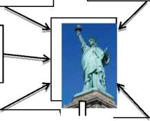
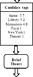
• Znaidia et al [11]. presented method for tag suggestion using visually similar images is given in figure 2. It consists in two main steps: creating a list of “candidate tags” from the visual neighbors of the untagged image then using them as pieces of evidence to be combined to provide the final list of predicted tags. Given an untagged image I, we start by searching the k nearest neighbors using
visual information (color,texture). First, we compute a BOW signature for each neighbor based on local soft coding. Second, a sum-pooling operation across the BOW of the k nearest neighbors is performed to obtain the list of “candidate tags” (the most frequent). Finally, basic belief masses are obtained for each nearest neighbour using the distances between this pattern and its neighbors. Their fusion leads to the list of final predicted tags.
-
• Verbeek et al [3]. proposed the weighted nearest neighbor for tag assignment as follows:
y. ^{ - 1, + 1 } to denote whether concept w is relevant for image i or not. The probability that concept w is relevant for image i, i.e. p ( y.w = + 1 ) , is obtained by taking a weighted sum of the relevance values for w of neighboring training images j. Formally, is defined as follows:
Р (У w = +1) = ^jjP ( y w = +1| j ) (9) j
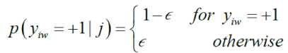
Where πij stands for the weight of training image j when it is predicting the annotation process for image i. to make sure that the distribution is carried out properly, require that n > 0 and£ n = 1.
Each term p ( y = + 1| j ) is the prediction according to neighbor j in the weighted sum. Neighbors predict that image I has got the same relevance for concept w with probability 1- Ɛ . The introduction of ǫ is a technique to avoid zero prediction probabilities when none of the neighbors j have the correct relevance value. The parameters of the model, which they will be introduce and below, control the weights. maximizing the log-likelihood of predicting correct annotations for training images in a leave-one-out manner helps to estimate the parameters. Excluding each training image, i.e. by setting π ii =0, as a neighbor of itself must be taken into account. The aim is to maximize т = ^ Ln P ( y ) .

Alex compos for music status Liberty

status Liberty

Status of Liberty Paris
Luxemburg
Canon 450d

Status
Liberty Nyc Strret Theater

Tag Local Soft Coding
Predicted tags
Status 0.99
Liberty 0.98 New York 0.97 Monument 0.95
Paris 0
Theater 0
Fig.2. an example of tags assignment based on belief theory and local coding.
• Li et al [10]. proposed TagVot algorithm for tag assignment. This method estimates the relationship of tag t in image X with the number of occurrence of t in the annotations of visual neighbors of X. This method introduces a unique user by limiting the neighbors to create more votings. Each user has got more than one image in neighbors set. Additionally, counting process of the occurrence of tags needs to be carried out in advance. This method is as follows:
j Tagvote ( x,t ) = kt - kn- (11)
Where n t is the number of tagged images with t tag in s set. K=1,000
-
• Chen, Fan, and Lin et al [9,14], proposed TagFeature method [9] for tag assignment. Enriching the feature of the images by adding an additional tag feature to each image is the core idea of this method. A tag word, which is composed of d', is the most number of frequent tags in s. Afterwards, a two-class linear SVM classifier is trained by LIBLINEAR. The positive training set includes p tagged images in S, the same amount of minus samples of training are randomly selected from untagged images. The output of the classifier, which is related to a special dimension in the tags of the image, is probably obtained by Platt scale. After adding tags and visual features, a feature is obtained by adding d+d' dimension. J TagFeature ( x , t ) is obtained for t test tag by retraining an SVM classifier by the help of added features. Being linear, the classifier groups all support vectors into one vector then tries to classify a test image by the help of this vector. This process is as follows:
j TagFeature ( x,t ) = b +< xt,x > (12)
Where Xt is the total weight of all supporting vectors and b is the intercept. In order to create meaningful classifiers tags having at least 100 positive samples are used. While d' is almost 400 [4,2] and p=500 and if the number of images for being tagged is more, a random vector sample is carried out.
-
B. Tag retr ev ng
-
• Liu et al [5], proposed two-phase tag ranking algorithm for tag retrieving. Given an image x and its tags, the first step produces an initial tag relevance score for each of the tags, obtained by (Gaussian) kernel density estimation on a set of ñ=1,000 images labeled with each tag, separately. Secondly, a random walk is performed on a tag graph where the edges are weighted by a tag-wise similarity. Then use the same similarity as in Semantic Field. Notice that when applied for tag retrieval, the algorithm uses the rank of t instead of
its score, i.e.,
J TagRanking (x, t) = - rank (t) +1 / lx where rank(t) returns the rank of t produced by the tag ranking algorithm. The term l/lx is a tiebreaker when two images have the same tag rank. Hence, for a given tag t, TagRanking cannot distinguish relevant images from irrelevant images if t is the sole tag assigned to them.
Table 4. A review of some sample based automatic image annotation methods in tag assignment.
|
Annotation method |
Providers |
Date & Location |
The aims of method |
|
local soft coding and belief theory |
Znaidia et all. |
April 16–20, 2013, Dallas, Texas, USA. |
|
|
A Weighted Nearest Neighbour Model |
Verbeek et all |
March 29–31, 2010, Philadelphia, Pennsylvania, USA. |
Using positive and negative samples of training with assuming the most relevant test tag t. Given the weight for neighbors |
|
TagVote |
Li et all |
ACM XXX X, X, Article X (March 2015) |
|
|
TagFeature |
Chen , Fan , Lin et all |
ACM XXX X, X, Article X (March 2015) |
|
-
• Guillaumin and Verbeek et al [2,3], proposed TagProp method. neighbor voting and distance parametric learning are used in this method. In this method a possible framework is proposed in which the probability of using neighboring images based on their rank or their weight according to their distance is defined. TagTop algorithm is as follows:
J TagProP ( x,t ) = y ^. I ( x , t )
Where π j is a non-negative weight indicating the importance of the j-th neighbor x j ,and I(x j ,t) returns 1 if x j is labeled with t, and 0 otherwise K=1,000 and the rank-based weights, which showed similar performance to the distance-based weights Differ from TagVote that uses tag prior to penalize frequent tags. Tag Prop promotes rare tags and penalizes frequent ones by training a logistic model per tag upon ^TagProp ( x,t ) . The use of the logistic model makes TagProp a modelbased method.
-
• Zhu et al [13], proposed graph voting. Graph voting is an oriented graph in which the nodes are annotated images by t tag in X. there e = ( i , j ) oE'.
exists, if and only if image i is in N k (i). X={x 1 ,x 2 ,…,x n ) is a set of feature vectors for all annotated images with t tag that xi ϵ Rd is the feature vector for ith image in X set and n is the number of annotated images by t tag. N k (i) refers to the K nearest neighbors of i based on parameters like Euclidian distance or cosine. It is worth noting that for calculating N k (i) not only annotated images by t are considered, but nonannotated image by t must be taken into account. The whole set of images is considered in order to find the K nearest neighbor set of Nk(i) for an image of i. Creating voting graph can be briefly described as follows: (1) For tag t, all annotated images having t tag are collected and used as the nodes of the graph. (2) the k nearest neighbors of N k (i) are obtained for each j image in X set in the whole set. If each I image in X set appear in N k (i), then there is an edge from vertex i to j. (3) the weight of W ij edge is set based on visual relevance between i and j. Visual relevance between two images is calculated by (Gaussian) kernel function with a parameter of ϭ diameter :
Wy = exp
II х , - x j || 2 '
-
• Makadia et al [1] used the K nearest neighbor for tag retrieving. This algorithm estimates the relationship of a tag by retrieving the first k nearest neighbor from S set based on visual distance d, then estimates the number of occurrence of the tag in the allocated neighbor tags. Knn is J KNN ( x , t ) : = kt • K t is the number of images with t tag in visual neighborhood of X.
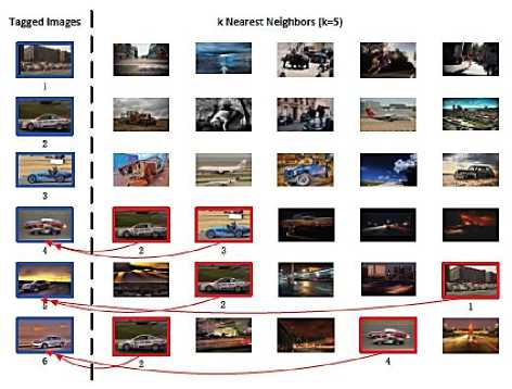
Fig.3. A sample of tag retrieving by voting graph method.
Table 5. A review of some sample based automatic image annotation methods in tag retrieving.
|
Annotation method |
Providers |
Date & Location |
The aims of method |
|
TagRanking |
Liu et all |
ACM XXX X, X, Article X (March 2015) |
|
|
TagProp |
Guillaumin , Verbeek et all |
ACM XXX X, X, Article X (March 2015) |
|
|
Vote graph |
Zhu et all |
July 6–11, 2014, Gold Coast, Queensland, Australia. |
|
|
k nearest neighbors |
Makadia , Ballan et all |
April 1–4, 2014, Glasgow, United Kingdom. |
estimates the relationship of a tag by retrieving the first k nearest neighbor from S set based on visual distance d, then estimates the number of occurrence of the tag in the allocated neighbor tags |
-
C. Tag refinement
-
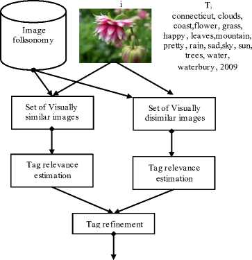
• Lee and Yong et al [17], proposed belief theory and neighbor voting for tag refinement in order to remove irrelevant tags among relevant ones. Let Ti is a set of allocated tags to i. Generally, Ti includes: (1) Relevant tags according to i content. (2) Irrelevant tags according to i content. During tag refinement if the relevance of a tag is less than a special threshold ξta g , T is irrelevant and T i is removed:
T rfed = {t 1 1 g T л r ( t , i ) > ^tag} (15)
Where T refined is a refined set of tags and ξtag determines if t is relevant or irrelevant according to i content. r(t,i)=rsimilar(t,i,k)-rdissimilar(t,i,l) where rsimilar(t,i,k) denotes the relevance of t with respect to I when making use of k folksonomy images visually similar to i, and rdissimilar(t,i,l) denotes the relevance of t with respect to i when making use of l folksonomy images visually dissimilar to i. (1) Neighbor voting is used in order to estimate rsimilar(t,i,k). The relevance of t based on i content is estimated as the difference among "annotated images with t in a set of k retrieved neighboring images of i from ranked images by the help of visual similarity search" and "number of annotated images with t in a set of k retrieved neighboring images of i from ranked images by the help of" random sampling method. (2) Visual dissimilarity is used in order to estimate rdissimilar(t,i,l). The relationship of t according to i content as the difference between "annotated images with t in a set of l images which are dissimilar to I is estimated. L images of ranked ones are retrieved by the help of visual dissimilarity search" and "annotated images with t are estimated in a set of l neighboring images which are retrieved by the help of random sampling method". The lower rdissimilar(t,i,l) is, the more t is related to i.
flower, grass, leaves
i

Fig.4. A sample of tag refinement by belief and neighbor voting method
-
• Van et al [15] proposed TagCooccur [7] method, which is based on tags, for tag retrieving. This method used the test rank of the tag in the list of tags ranking. The list is created by ordering all tags when they occur the tag simultaneously. this method also account for the calculated stabletag count through its occurrence.
-
• Zhu et al [16] proposed RobustPCA method [6]. This method is based on analyzing the main powerful factors, D matrix (tag and image) is factorization by analysis of low Rank decomposition with error scarcity and it is D=Ď+E in which Ď has a low rank constraint based on the nuclear norm, and E is an error matrix with l 1 -
- normsparsity constraint. Notice that this decomposition is not unique. The process of the image and tag nearness, as a solution, is carried out by adding two extra penalties with respect to a Laplacian matrix from the image affinity graph and another Laplacian matrix Lt from the tag affinity graph and it is relatively time consuming. Accordingly, two meta-parameters ʎ1 and ʎ2 are introduced in order to balance the error scarcity (two advantage of Laplacian). Two parameters are followed by a network search in the proposed area and a pretty stable algorithm is found. ʎ1=20 and ʎ2=2-10 are empirically selected. As the users' tags are usually lost, the researchers has proposed preprocessing phase in which D is valued with weighing Knn propagation based on visual similarity.
-
• Truong et al [17], proposed “Tag Influence-Unaware Neighbor Voting” method. In usual methods of voting all tags of the neighboring image of d' are supposed to have the same influence, according to the voting process, on describing visual contents of the image. For instance, relevance(tꞌ,dꞌ)=1, ⱯtꞌϵTdꞌ while the tags in a neighboring image tꞌϵT d ꞌ have various
applications in describing d'. However, it preferable to carry out the learning process for tag related to each dqD image. Afterwards, relevance(tꞌ,dꞌ)=1 (normalized[0,1]) is used for relearning related tag for a queried image. Notice that if the tag assignment compatible and its relationship are considered together, the noise can be identified easily. For instance, a tag like tꞌϵTdꞌ may be a little related to d', but it is vastly related to t voting. Accordingly, this refinement process is considered as precise compatibility of the tag.
Table 6. A review of some sample based automatic image annotation in tag refinement.
|
Annotation method |
Providers |
Date & Location |
The aims of method |
|
Belief Theory and Neighbor Voting |
Lee , Yong et all |
October 29, 2012, Nara, Japan |
belief theory and neighbor voting for tag refinement in order to remove irrelevant tags among relevant ones. the relevance of a tag is less than a special threshold |
|
TagCooccur |
Van et all |
ACM XXX X, X, Article X (March 2015) |
test rank of the tag in the list of tags ranking. The list is created by ordering all tags when they occur the tag simultaneously. account for the calculated stable tag count through its occurrence. |
|
RobustPCA |
Zhu et all |
July 6–11, 2014, Gold Coast, Queensland, Australia. |
analyzing the main powerful factors, D matrix (tag and image) is factorization by analysis of low Rankdecomposition with error scarcity |
|
Tag Influence-Unaware Neighbor Voting |
Troung et all |
12, June 5-8, Hong Kong, China |
Tag Influence-Unaware Neighbor Voting method. In usual methods of voting all tags of the neighboring image of d' are supposed to have the same influence, according to the voting process, on describing visual contents of the image |
-
IV. C ONCLUSION AND CHALLENGES
In spite of previous works on instance based automatic image annotation, it is still considered to be a challenge in this field. In this paper, instance based automatic image annotation methods were reviewed. The main parts of automatic image annotation and various similarity measures were firefly discussed. Afterwards, instance based automatic image annotation methods were discussed in three fields including assignment, refinement and retrieving of tags.
Being massive, the volume of the images in the dataset made the annotation algorithm to be time consuming. Volume and the number of created samples which is followed by neighboring estimation is a big challenge. Each above mentioned methods has advantages and disadvantages and rely on some specific feature of the images and they are defined based on data center and specific application. Having the methods combined increases the efficiency since they present more information about the image. Local features have a high differentiation power, but they are sensitive to noises and have less global differentiation power attributions and they are more stable than the noises.
The most important challenges in instance based automatic image annotation are as follows:
-
• The first challenge is to analyze the images with a high number of features. All features have limitations in interpreting the images and none of them can efficiently interpret the images of nature. Combining the features can be useful, but to analyze them is very complicated. Accordingly, choosing an suitable number of features seems to be essential in image annotating.
-
• The second challenge is to create an efficient model of annotating. Most current models learn from low level features of the images, but the number of samples for accurate training of a model is not big enough. Accordingly, texture information and metadata need to be used in annotating. How to combine both low level visual information and high level texture information together is a basic challenge.
-
• Today, annotation and online ranking are carried out simultaneously with several tags and they are not efficient enough in image retrieving. The solution is to do annotation offline with mono-tag method then to rank the tag separately. In this method, first, the image is annotated then it is ranked offline.
-
• The fourth challenge is the lack of standard and classified words for annotation. Now optional words are used. Consequently, it is not still clear that how the image is grouped. A hierarchical model of concepts is needed to accurately group the images.
-
• The next challenge is the weak tags of the images of the training set. Weak tag refers to tagged words and areas of the image that do not truly represent the content. For each image there are words that are tagged to the whole image and it is not clear which word refers to which area.
References A Review of Methods of Instance-based Automatic Image Annotation
- A. Makadia, V. Pavlovic, and S. Kumar. 2010. Baselines for Image Annotation. International Journal of Computer Vision 90, 1 (2010), 88–105.
- M. Guillaumin, T. Mensink, J. Verbeek, and C. Schmid. 2009. TagProp: Discriminative Metric Learning in Nearest Neighbor Models for Image Auto-Annotation. In Proc. of ICCV.
- J. Verbeek, M. Guillaumin, T. Mensink, and C. Schmid. 2010. Image annotation with TagProp on the MIRFLICKR set. In Proc. of ACM MIR.
- X. Li, C. Snoek, and M. Worring. 2009b. Learning Social Tag Relevance by Neighbor Voting. IEEE Transactions on Multimedia 11, 7 (2009), 1310–1322.
- D. Liu, X.-S. Hua, L. Yang, M. Wang, and H.-J.Zhang. 2009. Tag Ranking. In Proc. of WWW.
- G. Zhu, S. Yan, and Y. Ma. 2010. Image Tag Refinement Towards Low-Rank, Content-Tag Prior and Error Sparsity. In Proc. of ACM Multimedia.
- K. van de Sande, T. Gevers, and C. Snoek. 2010. Evaluating Color Descriptors for Object and Scene Recognition. IEEE Transactions on Pattern Analysis and Machine Intelligence 32, 9 (2010), 1582–1596.
- J. Sang, C. Xu, and J. Liu. 2012. User-Aware Image Tag Refinement via Ternary Semantic Analysis. IEEE Transactions on Multimedia 14, 3 (2012), 883–895.
- L. Chen, D. Xu, I. Tsang, and J. Luo. 2012. Tag-Based Image Retrieval Improved by Augmented Features and Group-Based Refinement. IEEE Transactions on Multimedia 14, 4 (2012), 1057–1067.
- X. Li and C. Snoek. 2013. Classifying tag relevance with relevant positive and negative examples. In Proc. of ACM Multimedia.
- A. Znaidia, H. Le Borgne, and C. Hudelot. 2013. Tag Completion Based on Belief Theory and Neighbor Voting. In Proc. of ACM ICMR.
- Z. Lin, G. Ding, M. Hu, J. Wang, and X. Ye. 2013. Image Tag Completion via Image-Specific and Tag-Specific Linear Sparse Reconstructions. In Proc. of CVPR.
- X. Zhu, W. Nejdl, and M. Georgescu. 2014. An Adaptive Teleportation Random Walk Model for Learning Social Tag Relevance. In Proc. of SIGIR.
- Y. Yang, Y. Gao, H. Zhang, J. Shao, and T.-S. Chua. 2014. Image Tagging with Social Assistance. In Proc. Of ACM ICMR..
- K. van de Sande, T. Gevers, and C. Snoek. 2010. Evaluating Color Descriptors for Object and Scene Recognition. IEEE Transactions on Pattern Analysis and Machine Intelligence 32, 9 (2010), 1582–1596.
- G. Zhu, S. Yan, and Y. Ma. 2010. Image Tag Refinement Towards Low-Rank, Content-Tag Prior and Error Sparsity. In Proc. of ACM Multimedia.
- B. Truong, A. Sun, and S. Bhowmick. 2012. Content is still king: the effect of neighbor voting schemes on tag relevance for social image retrieval. In Proc. of ACM ICMR.
