A Soil Nutrient Assessment for Crop Recommendation Using Ensemble Learning and Remote Sensing

Understanding and managing soil nutrients, such as nitrogen (N), phosphorus (P), potassium (K), and pH, is crucial in addressing soil variability challenges and climate uncertainty [1]. This knowledge not only increases plant resilience to climate change and water use efficiency [1,2], but also plays a vital role in plant growth. A balanced soil pH, for instance, significantly affects the availability of nutrients [2,3]. In the face of increasing climate uncertainty, a dynamic and adaptive approach to agriculture is essential. Understanding and managing soil nutrients enables farmers to be more responsive to changing climatic conditions, thereby reducing the risk of environmental stress on plants, and enhancing growth and productivity.

Proper nutrition management is a solution to the phenomenon of climate change [4]. Knowledge of the nutrient status of the soil allows for more effective use of water as well as fertilizer, minimizing resource waste and ensuring that plants get enough moisture and fertilizer for optimal growth [3]. However, many agricultural practices still do not integrate soil nutrient analysis in depth, leading to inefficient use of inputs. This condition not only has an impact on crop yields but also environmental sustainability. Thus, understanding the suitability of soil nutrients becomes the foundation for responsible and sustainability-oriented agricultural planning.

Soil nutrients have an impact on the type of crops to be planted [5]. Each plant has specific nutrient needs, and choose plants that fit the required soil nutrient profile [4,6]. For example, plants that require high levels of nitrogen will thrive better in nitrogen-rich soils. Similarly, the pH level of the soil helps determine which plants will grow more effectively. Thus, determining the type of plant according to nutrition is an important part of agricultural planning, ensuring that the selected plants are suitable for the soil environment. Appropriate planning can maximize the efficiency of resource use and crop yields. So, for ideal planning, the integration of artificial intelligence-based technology and remote sensing, which is called precision agriculture, is needed. The integration of precision agriculture technology with a deep understanding of soil nutrients and local climatic conditions allows for more adaptive and responsive agricultural systems to environmental changes.

In the previous study, utilizing computational intelligence using ensemble learning was used to classify images of rice fields [7]. Then, the application of Machine Learning for plant recommendations [8]. Another study uses remote sensing and machine learning for soil nutrient prediction [9] and mapping classification [10,11]. This proves that computational intelligence and remote sensing provide opportunities to support precision agriculture.

Computational intelligence allows for more accurate and predictive data analysis of various agricultural parameters [12]. Techniques in computational intelligence can process and analyze large and complex amounts of data, such as soil nutrient data, weather conditions, and satellite imagery, to produce timely and location-specific recommendations for farmers [13]. Additionally, computational intelligence can improve resource management, which can ultimately reduce operational costs and improve production yields [12]. Meanwhile, Remote sensing, which involves the use of satellite imagery and aerial sensors, provides extensive data [14]. This technology allows for continuous monitoring of plant health, soil moisture, and nutrient levels on a wide scale [13]. Thus, the combination of computational intelligence and remote sensing creates an integrated precision agriculture system that supports sustainable agricultural practices that can adapt to climate change. Therefore, this research proposes a soil nutrient assessment that can recommend plant types using ensemble learning and remote sensing to support precision agriculture. With this approach, farmers can more quickly adjust the type of crops to be planted with the soil nutrient conditions on-site.

This article describes the role of precision agriculture in supporting modern agriculture. Then, the materials and methods used, the proposed scheme in the integration of prediction of plant type adaptation through computational intelligence and remote sensing. Finally, the conclusion and recommendations of the findings for future research.

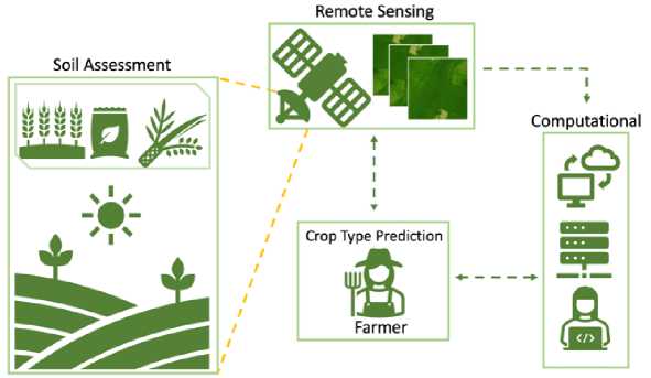
Fig.1. Precision agriculture scheme by combining computational intelligence and remote sensing

2.    Precision Agriculture Overview

Precision agriculture has the opportunity to be applied in optimizing the use of agricultural resources; by using precision agriculture technology, farmers can monitor plant conditions in real time through remote sensing data, as shown in Figure 1. The information obtained from this remote sensing can provide a better understanding of soil conditions, moisture, nutrient needs, and crop yield estimates. Then, the phenomenon of climate change demands more modern and sustainable agricultural management.

On the other hand, the science of "niten", or traditional knowledge of local weather patterns, crop cycles, and adaptation to environmental conditions, has not been able to help farmers make better decisions in the face of climate change. Thus, it is necessary to support the traditional knowledge of farmers with precision agriculture technology to face the challenges of climate change, increase agricultural productivity, and maintain environmental sustainability using ensemble learning and remote sensing.

According to several studies, the use of remote sensing and artificial intelligence in precision agriculture has shown significant results such as mapping [15], monitoring plant health [16] and prediction of crop yield [17]. Remote sensing and artificial intelligence (AI) in precision agriculture are significant advances in modern agricultural technology, offering great potential to improve efficiency, productivity, and sustainability in global agricultural practices. In addition, the integration of artificial intelligence and remote sensing technologies can optimize resource use and improve crop yields through data analysis at scale and high speed. AI is used to process data collected from various sources, including soil conditions, with satellite imagery to provide precise and real-time recommendations to farmers [18,19].

Remote sensing also plays an important role in land mapping, monitoring plant conditions, and early detection of diseases and pests. Satellite imagery also allows for the collection of detailed data on plant health, soil moisture, and fertilization needs [20]. The combination of AI and remote sensing enables predictive analytics that can help farmers make smarter and more timely decisions, reduce operational costs, and improve productivity and environmental sustainability.

3.    Related Works

Plant recommendations using machine learning (ML) and remote sensing techniques show that the methods used are very diverse, ranging from deep learning models (DNNs) to various ensemble learning techniques. For example, a study using the Wrapper-PART-Grid model for crop recommendation optimization showed high reliability and accuracy, reaching 99.31% [21]. Another study using a DNN-based GBRT replacement model also showed high accuracy with an F1 score of 1.0 [19]. This study shows that soil data management and the development of appropriate prediction models are essential to improve agricultural productivity through accurate crop recommendations.

Furthermore, studies in India have shown that the integration of multispectral remote sensing data with machine learning models has practical implications for estimating soil nutrient content [22,23]. The use of data from Landsat 8 and Sentinel-2 to estimate nutrients such as N, P, and K shows that ensemble models such as Gradient Boosting and Random Forest Regression give good results with sMAPE in the range of 0.125-0.377 [9]. Another study in the Punjab region, northern India, also showed that remote sensing data can be used to accurately estimate soil texture and nutrient content using various ensemble learning methods, highlighting the practical relevance of these techniques [24].

However, despite the various approaches that have been developed, several study gaps still need to be addressed. First, most of the existing research focuses on the technical aspects and performance of the model but needs more practical integration and adoption of conditions in the field. Second, there is a need to explore further the potential for combining remote sensing data with other soil condition data, such as temperature and humidity, to provide more holistic recommendations. Thus, the proposed study "Soil Nutrient Assessment for Plant Recommendations Using Ensemble Learning and Remote Sensing" can make a significant contribution. By combining proven effective ensemble learning techniques with remote sensing data, this research can not only improve accuracy in soil nutrient assessment but also offer a more practical and holistic scheme for precision agriculture. The use of remote sensing allows for a broad and continuous assessment of soil conditions. At the same time, ensemble learning techniques ensure accuracy in plant type recommendations, providing a more integrated solution to support farmers' decisions in their daily farming practices.

4.    Materials and Methods

The study proposes a scheme for soil nutrient assessment that aims to provide plant recommendations by utilizing Ensemble Learning and Remote Sensing techniques. Through this approach, a framework that integrates intelligent data processing (computational intelligence) with remote sensing technology is proposed.

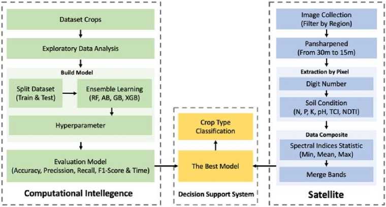
Fig.2. Flow of soil nutrient assessment scheme and integration of intelligent computing and remote sensing

The flow of the study is illustrated in Figure 2, which shows the soil nutrient assessment scheme and the integration between intelligent computing and remote sensing. The process begins with the collection of data from a variety of sources, including satellite imagery and nutritional tabular data. The data is then trained using ensemble learning.

The integration of Computational and Remote Sensing used in this study involves several stages, including thorough data pre-processing, feature extraction, and model training. Data pre-processing is meticulously carried out to clean and prepare the data so that it is ready for further analysis. Feature extraction is then performed to identify and extract important features from data related to soil nutrients.

Once the critical features are identified, the data is trained using several different Machine Learning models, showcasing the study's adaptability. The results of the model are then used to provide recommendations for plants that are most suitable for soil conditions. The integration between intelligent computing and remote sensing allows soil nutrient assessments to be carried out more measurably. Remote sensing technology provides extensive and detailed data on soil conditions from different regions, while Ensemble Learning techniques ensure data analysis is carried out in-depth and on target.

• 4.1.    Data Collection

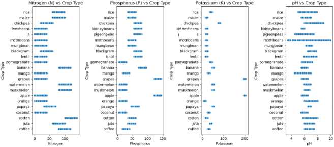
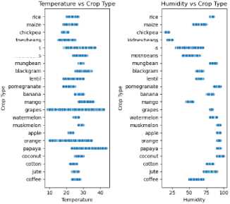
Model training data in the form of tabular data accessed on the Government of India's website from soil testing sensors data has been collected from several regions of India [25]. This data reflects conditions in Indonesia, which also has a tropical climate, although some areas of India have a subtropical climate. The parameter used nitrogen (N) reflects the ratio of Nitrogen content in soil; phosphor (P) ratio of Phosphorous content in soil; Potassium (K) ratio of Potassium content in soil; Temperature (C) temperature in degrees Celsius; Humidity (H) relative humidity in %; and acid (pH) ph value of the soil (Figure 3). The dataset consists of 22 types of plants (can be seen in Figure 4), such as (rice, maize, jute, cotton, coconut, papaya, orange, apple, muskmelon, watermelon, grapes, mango, banana, pomegranate, lentil, black gram, mungbean, moth beans, pigeon peas, kidney beans, chickpea, and coffee) each class has a total of 100 distributions.

kidneybeans pigeonpeas mothbeans kidney beans ptgeonpeas moth beans

Fig.3. Distribution of soil nutrient attributes by plant type

u pomegranate

kidneybeans pigeonpeas mothbeans

kidneybeans pigeonpeas mothbeans

Distribution of Crop Types rice -| maize -1 chickpea -| kidneybeans ~| pigeonpeas -| mothbeans -| mungbean -| blackgram -| lentil -| pomegranate -| ф     banana-^И ф     mango-^H grapes ~H watermelon muskmelon apple orange papaya coconut - В cotton -___ jute -____ coffee -

0                20                40                60                80               100

Count

Fig.4. Distribution of plant type datasets

Meanwhile, remote sensing data uses area of interest data in the Banyumas area, as seen in Figure 5. The Banyumas area was chosen with the consideration of regional topology, which includes mountains, rural and urban.

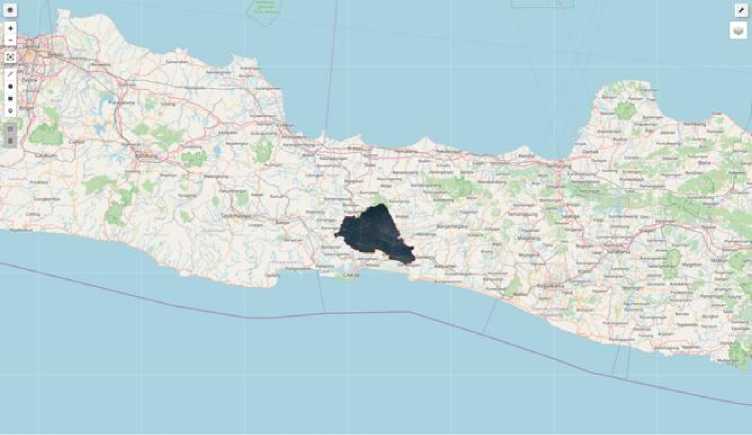
Fig.5. Regional locations for nutrition assessment in Banyumas, Central Java, Indonesia

Furthermore, remote sensing data was taken using the Landsat 8 Top of Atmosphere reflectance satellite from 2015 to 2018. It was then sharpened from 30m to 15m (Figure 6) using the pansharpening technique, which combined the panchromatic band as per Formula 1.

R out (

R in

' ^Rin + ^G in + ^B in

Л *P-

) in

where, R_in = Band 4 (Red), G_in = Band 3 (Green), B_in= Band 2 (Blue), and P_in = Band 8 (panchromatic).

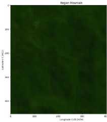
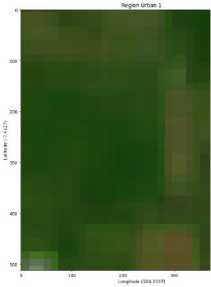
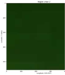
Figure 7 is an area of interest that consists of mountainous areas, urban areas, and rural areas. Then, the area of interest is assessed for the suitability of soil nutrients based on feature extraction through integration with computational intelligence.

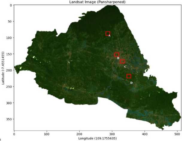
Fig.6. Banyumas region that has been pansharped and the position of the area of interest

• 4.2.    Ensemble Learning Model

Ensemble learning is a technique in machine learning in which multiple models (e.g., classifiers) are combined to produce better predictions compared to a single model. This method takes advantage of the diversity of models used to reduce variance, bias, or increase generalization. There are various ensemble learning techniques, including bagging (Random Forest) and boosting (AdaBoost and Gradient Boosting). This technique can significantly improve model performance, especially in situations where data has high complexity and non-linearity. According to [26], ensemble methods have shown superior performance in various tasks and are considered one of the most powerful tools in the machine learning toolkit.

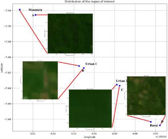
Fig.7. Sample datasets in areas of interest such as mountains, urban and rural areas

• A.    Random Forest Algorithm

Random Forest, an ensemble learning method, is used for classification, regression, and other tasks. It operates by building multiple decision trees during training, and the output is either the mode of class (classification) or prediction average (regression) of each tree. Each tree in a random forest is constructed from a bootstrap sample of training data. At each split node, a 'randomly selected subset of features' is considered for the best split. This feature selection process is crucial as it helps to reduce overfitting and improve model generalization [27]. The formula for random forests in the classification can be expressed by Formula 2.

ул = mode{h i (x), h 2 (x),..., h_B(x)}                                    (2)

where h 1 (x), h₂ (x) is the prediction of the i-th tree, and В is the total number of trees in the forest.

• B.    AdaBoost Algorithm

AdaBoost (Adaptive Boosting) is an ensemble method that improves classification accuracy by combining a number of weak learners, usually a single-level decision tree. The algorithm operates by training the model sequentially, where each subsequent model tries to correct the errors made by the previous model. Each observation is weighted, and this weight is adjusted at each iteration to emphasize observations that are difficult to classify. Ultimately, the final prediction is made by combining the predictions of all weak learning models with the corresponding weights [28], as per Formula 3.

H ⁽x) = sign(^^₌₁ a_tH_t⁽x))                                      (3)

where a_t is the weight of the t-th weak learning model, H_t(x') is the prediction of thet-th model, and T is the total sum of the models.

• C.    Gradient Boosting Algorithm

Gradient Boosting is an ensemble method that combines multiple weak learners, such as decision trees, to form a strong model. This algorithm works by building the model incrementally, where each new model seeks to correct the residual errors made by the previous model. This process involves optimizing the loss function using the gradient descent method. With each iteration, a new model is added to minimize the loss function by pointing the model in the direction of the negative gradient of the error. The basic formula for prediction on Gradient Boosting is [29], as is Formula 4.

F_m(x)=F_m - ₁(x) + v-H_m(x)                                (4)

where F_m(x) is the model generated in the m -th iteration, F_m-1(x) is the model in the previous iteration, v is the learning rate, and H_m(x) is a weak learning model generated in the m-th iteration.

• D.    XGBoost Algorithm

• 4.3.    Extraction of Soil Condition Features

5.    Results and Discussion

XGBoost (Extreme Gradient Boosting) is an enhancement algorithm of Gradient Boosting that is optimized for performance and efficiency. XGBoost is designed to overcome some of the drawbacks of Gradient Boosting by providing faster training speeds, scalability, and the ability to handle big data. The algorithm implements robust treebased optimization and uses regularization techniques (L1 and L2) to reduce overfitting, as well as parallelization to speed up the training process. XGBoost also supports data sparsity management and feature grouping which helps in handling incomplete or very large data. This model updates the predictions by adding a new decision tree that corrects the residual errors from the previous model in a similar way to Gradient Boosting. The basic formula for model updates is Formula 5 [30].

F m (x) = F m-1 (X) + t] ' h m (x)                                     (5)

where Fn(x) is the model in the m-th iteration, F_m-1(x') is the model in the previous iteration, ] is the learning rate, and h_m (x) is a weak learning model added to the m-th iteration.

The integration between ensemble learning and remote sensing data requires the extraction of soil condition features. These features are obtained from various input data sourced from Landsat 8 satellite image extraction. For example, to extract the nitrogen (N) content, the model uses a combination of various wavelengths of light such as blue, green, red, NIR (near-infrared), SWIR1, and SWIR2. In the feature extraction, the focus is on the values of N, P, K, pH, Temperature (TCI) and Humidity (NDTI) with the formula as shown in Table 1.

Table 1. Predicted performance summary of out of school children trend rate data using the MLP-NN model using different training algorithms

Attributes Formula N [31] = -31.661 + 186.022 x Blue - 364.274 x Green + 421.943 x Red - 308.068 x NIR + 207.957 x SWIR1 - 12.762 x SWIR2 P [31] = 0.404 - 2.702 x Blue + 22.540 x Green - 14.156 x Red + 3.613 x NIR - 2.648 x SWIR1+ 2.304 x SWIR2 K [31] = -610.060 - 1424.543 x Red + 933.043 x SWIR2 + 4103.577 x Green - 1733.486 x Blue Ph [31] = 3.983 - 0.544 x Blue - 1.112 x Green + 6.131 x Red + 2.193 x NIR - 1.647 x SWIR1 + 2.739 x SWIR2 TCI (Temperature Condition Index) [32] = 100 * (BTmax - BT) / (BTmax - BTmin) NDTI (Normalized Difference Turbidity Index) [33] = (Red - Green) / (Red + Green) where Blue = Band 2, Green = Band 3, Red = Band 4, NIR = Band 5, SWIR1 = Band 6, SWIR2 = Band 7, BTmax is the maximum brightness temperature, BTmin is the minimum brightness temperature, and BT is the current brightness temperature.

This section discusses the results of classification model and the proposed integration computational intelligence and remote sensing.

• 5.1.    Classification Model

  This analysis evaluates the performance of various classification models by using GPU-PyTorch hardware, which has 4 cores and 28 GiB of memory. The models used include Random Forest, Gradient Boosting, AdaBoost, and XGBoost, with each model set with various parameters to measure accuracy, recall, F1 score, precision, and execution time, as shown in Table 2, Table 3, Table 4, and Table 5. The Random Forest algorithm exhibits outstanding effectiveness with relatively fast computing times. After experimenting with various combinations of parameters such as n_estimators , max_features , max_depth , and criterion , we identified the best configuration as n_estimators 150, max_features 'log2', max_depth 10, and criterion 'entropy'. This setup delivers high accuracy, recall, F1 score, and precision, approximately 0.9772, 0.9772, 0.9776, and 0.9802, respectively, with a compute time of 0.89 seconds. This strong performance underscores the reassurance we can derive from the Random Forest algorithm for classification tasks with the right parameters.

Table 2. Ensemble learning by random forest

Hyperparameter	Accuracy	Recall	F1 Score	Precision	Elapsed Time (s)
'n_estimators': 50, 'max_features': 2, 'max_depth': 10, 'criterion': 'gini'	0.9704	0.9704	0.9706	0.9734	0.6609
'n_estimators': 50, 'max_features': 'sqrt', 'max_depth': 10, 'criterion': 'gini'	0.9704	0.9704	0.9706	0.9734	0.5454
'n_estimators': 50, 'max_features': 'log2', 'max_depth': 10, 'criterion': 'gini'	0.9704	0.9704	0.9706	0.9734	0.4297
'n_estimators': 50, 'max_features': 2, 'max_depth': 10, 'criterion': 'entropy'	0.9681	0.9681	0.9682	0.9713	0.7404
'n_estimators': 50, 'max_features': 'sqrt', 'max_depth': 10, 'criterion': 'entropy'	0.9681	0.9681	0.9682	0.9713	0.7223
'n_estimators': 50, 'max_features': 'log2', 'max_depth': 10, 'criterion': 'entropy'	0.9681	0.9681	0.9682	0.9713	0.6181
'n_estimators': 100, 'max_features': 2, 'max_depth': 10, 'criterion': 'gini'	0.9681	0.9681	0.9684	0.9710	1.1128
'n_estimators': 100, 'max_features': 'sqrt', 'max_depth': 10, 'criterion': 'gini'	0.9681	0.9681	0.9684	0.9710	1.5361
'n_estimators': 100, 'max_features': 'log2', 'max_depth': 10, 'criterion': 'gini'	0.9681	0.9681	0.9684	0.9710	1.7131
'n_estimators': 100, 'max_features': 2, 'max_depth': 10, 'criterion': 'entropy'	0.9750	0.9750	0.9752	0.9777	2.4873
'n_estimators': 100, 'max_features': 'sqrt', 'max_depth': 10, 'criterion': 'entropy'	0.9750	0.9750	0.9752	0.9777	2.3306
'n_estimators': 100, 'max_features': 'log2', 'max_depth': 10, 'criterion': 'entropy'	0.9750	0.9750	0.9752	0.9777	2.0949
'n_estimators': 150, 'max_features': 2, 'max_depth': 10, 'criterion': 'gini'	0.9727	0.9727	0.9730	0.9752	2.2085
'n_estimators': 150, 'max_features': 'sqrt', 'max_depth': 10, 'criterion': 'gini'	0.9727	0.9727	0.9730	0.9752	2.3797
'n_estimators': 150, 'max_features': 'log2', 'max_depth': 10, 'criterion': 'gini'	0.9727	0.9727	0.9730	0.9752	2.2019
'n_estimators': 150, 'max_features': 2, 'max_depth': 10, 'criterion': 'entropy'	0.9772	0.9772	0.9776	0.9802	3.9282
'n_estimators': 150, 'max_features': 'sqrt', 'max_depth': 10, 'criterion': 'entropy'	0.9772	0.9772	0.9776	0.9802	2.2019
'n_estimators': 150, 'max_features': 'log2', 'max_depth': 10, 'criterion': 'entropy'	0.9772	0.9772	0.9776	0.9802	2.2019

Table 3. Ensemble learning by gardient boosting

Hyperparameter	Accuracy	Recall	F1 Score	Precision	Elapsed Time (s)
'n_estimators': 50, 'learning_rate': 0.1, 'max_depth': 10	0.9409	0.9409	0.9439	0.9520	17.2418
'n_estimators': 50, 'learning_rate': 0.01, 'max_depth': 10	0.9227	0.9227	0.9328	0.9559	19.5301
'n_estimators': 50, 'learning_rate': 0.001, 'max_depth': 10	0.9272	0.9272	0.9371	0.9618	17.5320
'n_estimators': 100, 'learning_rate': 0.1, 'max_depth': 10	0.9431	0.9431	0.9442	0.9489	26.9073
'n_estimators': 100, 'learning_rate': 0.01, 'max_depth': 10	0.9318	0.9318	0.9390	0.9593	42.4835
'n_estimators': 100, 'learning_rate': 0.001, 'max_depth': 10	0.9272	0.9272	0.9218	0.9618	19.9181
'n_estimators': 150, 'learning_rate': 0.1, 'max_depth': 10	0.9431	0.9431	0.9448	0.9489	28.7553
'n_estimators': 150, 'learning_rate': 0.01, 'max_depth': 10	0.9340	0.9340	0.9415	0.9611	61.9243
'n_estimators': 150, 'learning_rate': 0.001, 'max_depth': 10	0.9250	0.9250	0.9353	0.9590	55.3269

Meanwhile, Gradient Boosting shows a longer computing time than Random Forest, ranging from 17 to 60 seconds, but is able to achieve good performance with certain configurations. The combination of n_estimators 50, learning_rate 0.1, and max_depth 10 resulted in the best performance with accuracy, recall, F1 score, and precision of around 0.940, 0.940, 0.943, and 0.952, respectively. Although the compute time is higher, Gradient Boosting can provide excellent results if time is not the main constraint. Meanwhile, AdaBoost has a faster compute time than Gradient Boosting, ranging from 1 to 4 seconds, and provides consistent performance results. The combination of n_estimators 150, learning_rate 0.001, and base_estimator with max_depth 10 resulted in the best performance with accuracy, recall, F1 score, and precision of around 0.968, 0.968, 0.968, and 0.9706.

Furthermore, XGBoost delivers excellent performance with relatively short computing times, demonstrating superiority in computing efficiency and performance. With n_estimators 100, learning_rate 0.1, max_depth 10, and random_state 42 configurations, XGBoost achieves accuracy, recall, F1 score, and precision of around 0.970, 0.972, 0.969, and 0.968 respectively with a computing time of just 0.706 seconds. This result shows that XGBoost is capable of delivering excellent results with high time efficiency, making it a superior choice for applications with fast computing and high-performance requirements.

Table 4. Ensemble learning by adaboost

Hyperparameter	Accuracy	Recall	F1 Score	Precision	Elapsed Time (s)
'n_estimators': 50, 'learning_rate': 0.1, 'base_estimator': DecisionTreeClassifier(max_depth=10), 'random_state': 42	0.9409	0.9409	0.9417	0.9465	0.8479
'n_estimators': 50, 'learning_rate': 0.01, 'base_estimator': DecisionTreeClassifier(max_depth=10), 'random_state': 42	0.9659	0.9659	0.9661	0.9672	0.8356
'n_estimators': 50, 'learning_rate': 0.001, 'base_estimator': DecisionTreeClassifier(max_depth=10), 'random_state': 42	0.9613	0.9613	0.9617	0.9662	0.8888
'n_estimators': 100, 'learning_rate': 0.1, 'base_estimator': DecisionTreeClassifier(max_depth=10), 'random_state': 42	0.9409	0.9409	0.9417	0.9465	0.8401
'n_estimators': 100, 'learning_rate': 0.01, 'base_estimator': DecisionTreeClassifier(max_depth=10), 'random_state': 42	0.9545	0.9545	0.9549	0.9573	1.6387
'n_estimators': 100, 'learning_rate': 0.001, 'base_estimator': DecisionTreeClassifier(max_depth=10), 'random_state': 42	0.9681	0.9681	0.9684	0.9706	1.6875
'n_estimators': 150, 'learning_rate': 0.1, 'base_estimator': DecisionTreeClassifier(max_depth=10), 'random_state': 42	0.9409	0.9409	0.9417	0.9465	0.9957
'n_estimators': 150, 'learning_rate': 0.01, 'base_estimator': DecisionTreeClassifier(max_depth=10), 'random_state': 42	0.9568	0.9568	0.9572	0.9592	3.5680
'n_estimators': 150, 'learning_rate': 0.001, 'base_estimator': DecisionTreeClassifier(max_depth=10), 'random_state': 42	0.9681	0.9681	0.9684	0.9706	2.7145

Table 5. Ensemble learning by XGBoost

Hyperparameter	Accuracy	Recall	F1 Score	Precision	Elapsed Time (s)
'n_estimators': 50, 'learning_rate': 0.1, 'max_depth': 10, 'random_state': 42	0.9681	0.9707	0.9671	0.9660	0.4364
'n_estimators': 50, 'learning_rate': 0.01, 'max_depth': 10, 'random_state': 42	0.9590	0.9629	0.9587	0.9580	0.4940
'n_estimators': 50, 'learning_rate': 0.001, 'max_depth': 10, 'random_state': 42	0.9409	0.9453	0.9695	0.9410	0.4385
'n_estimators': 100, 'learning_rate': 0.1, 'max_depth': 10, 'random_state': 42	0.9704	0.9726	0.9697	0.9688	0.7060
'n_estimators': 100, 'learning_rate': 0.01, 'max_depth': 10, 'random_state': 42	0.9613	0.9644	0.9606	0.9605	0.8822
'n_estimators': 100, 'learning_rate': 0.001, 'max_depth': 10, 'random_state': 42	0.9454	0.9491	0.9445	0.9453	0.8606
'n_estimators': 150, 'learning_rate': 0.1, 'max_depth': 10, 'random_state': 42	0.9704	0.9726	0.9697	0.9688	0.8869
'n_estimators': 150, 'learning_rate': 0.01, 'max_depth': 10, 'random_state': 42	0.9636	0.9672	0.9625	0.9617	1.3351
'n_estimators': 150, 'learning_rate': 0.001, 'max_depth': 10, 'random_state': 42	0.9454	0.9495	0.9450	0.9458	1.2968

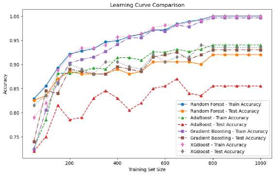
Fig.8. Comparison of performance of the four ensemble learning algorithms

Overall, if the top priority is fast computing time with high performance, XGBoost and Random Forest are superior choices. AdaBoost also shows good performance with relatively fast computing times, which is suitable for applications with performance consistency requirements. In contrast, Gradient Boosting offers strong performance, albeit with higher compute times, and can be a good option when performance is a top priority over time. Each algorithm has its strengths, and the right choice must take into account the specific needs of the application to be used, as seen in Figure 8 and Figure 9, where the performance comparison between the four algorithms is shown. So, the dominant ensemble algorithms are Random Forest and XGBoost. However, in the Ensemble algorithm, which is integrated with remote sensing data in this research, paying attention to reliability and time efficiency, Random Forest is an option to be used in soil nutrient assessment on remote sensing image data.

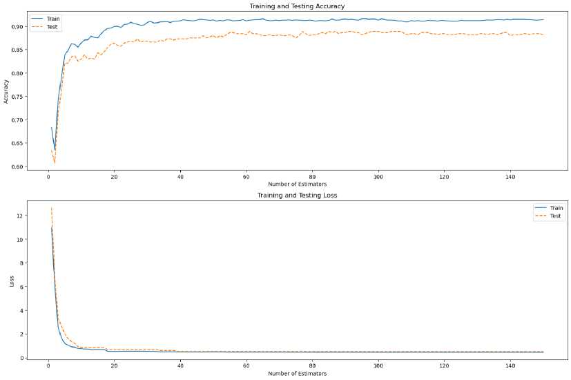
Fig.9. Random Forest evaluation results from the best performance of the four ensemble learning algorithms

5.2. Proposed Integration Computational Intelligence and Remote Sensing

After obtaining the best model results, the integration between computational intelligence and remote sensing is carried out first to extract features in each region. The results of the region extraction are seen in Figure 10.

Mountain:

AVA_N   AVAP      AVA_K      pH      TCI    NDTI      Long      Lat

0   -50.382234  1.589334 -466.997635 4.147764  11.339976 0.769273  109.203556 -7.338852

1   -50.403278  1.590667 -466.836831  4.147949  11.339976 0.769273  109.203556  -7.338852

2   -46.741340  1.367250 -505.522191  4.121569  11.340230 0.718488  109.203556  -7.338852

3   -46.419578  1.346698 -507.752668  4.118612  11.340230 0.718488  109.203556 -7.338852

4   -43.074523  1.115778 -541.132474 4.089840 11.340367 0.650951  109.203556  -7.338852

2845 -56.385425 2.038232 -416.508693 4.230377  11.339888 0.638514  109.203556 -7.338852

2846 -55.351776  1.997701  -420.796923 4.234535  11.339937 0.591727  109.203556 -7.338852

2847 -51.579402  1.743930 -450.934015 4.194482  11.339937 0.591727  109.203556 -7.338852

2848  -49.674171  1.546993 -482.633332 4.147228  11.339897 0.654654  109.203556  -7.338852

2849  -46.828974  1.366456 -502.760500 4.121288 11.339897 0.654654  109.203556 -7.338852

2850 rows x 8 columns Urban 1:

AVA_N   AVA_P      AVA_K      pH      TCI    NDTI      Long      Lat

0   -42.923714  1.428339  -486.509716 4.241863  11.324317 0.392659  109.232577 -7.411433

1   -43.295822  1.462182 -482.427750 4.250416  11.324317 0.392659  109.232577 -7.411433

2   -51.235148  1.716943  -454.166985 4.189652  11.325709 0.596102  109.232577 -7.411433

3   -50.398755  1.660841  -460.828203 4.180822  11.325709 0.596102  109.232577 -7.411433

4   -51.891160  1.604813 -474.606332 4.143360  11.326830 0,761584  109,232577 -7,411433

318 -51.454149  1.660547  -462.298809  4 168810  11.330563 0.696751  109.232577 -7.411433

319 -52.282513 1.713135 -456.114854 4 176586 11.330563 0 696751  109.232577 -7 411433

320 -53.603921 1.796187 -445.425812 4.191966 11.331024 0.702108 109.232577 -7.411433

321  -55.070836  1.889256 -434.419779 4.205936  11.331024 0.702108  109.232577 -7.411433

322 -54.619035  1.911905 -419.737552  4 211560  11.331427 0.699901  109.232577 -7.411433

323 rows x 8 columns

Urban 2: AVA_N		AVA_P	AVA_K	pH	TCI	NDTI	Long	Lat
0	-36.493022	1.370310	-448.721083	4.390449	11.329070	0.248413	109.251032	-7.435524
1	-42.107688	1.595342	■453.408086	4.319553	11.329596	0.356162	109.251032	-7.435524
2	-41.997661	1.582795	-455.057974	4.316008	11.329596	0.356162	109.251032	-7.435524
3	-41.375118	1.533685	-461.960358	4.305669	11.329635	0.349909	109.251032	-7.435524
4	-41.150448	1.507558	-465.385630	4 298206	11.329635	0.349909	109.251032	-7.435524
85	-40.337000	1.738360	-415.975686	4.408524	11.327535	0.318369	109.251032	-7.435524
86	-40.015907	1.688977	-423.158641	4.392776	11.327535	0.318369	109.251032	-7.435524
87	-39.730109	1.630323	-436.317781	4.368881	11.327125	0.318497	109.251032	-7.435524
88	■39.372141	1.575920	■444.025409	4.351763	11.327125	0.318497	109.251032	-7.435524
89	-39.430436	1.659244	-424.110022	4.388773	11.326726	0.316454	109.251032	-7.435524

Fig.10. Pixel-based extraction of soil nutrient value

90 rows x 8 columns Rural:

	AVA_N	AVA_P	AVA_K	pH	TCI	NDTI	Long	Lat
0	-48.007996	1.808962	-417.724359	4.272056	11.330285	0.537701	109.267667	-7.483373
1	-48.189312	1.824546	-415.591033	4.275262	11.330285	0.537701	109.267667	-7.483373
2	-42.500579	1.623326	-440.639465	4.293575	11.330544	0.425516	109.267667	-7.483373
3	-42.541979	1.627983	-439.992416	4.294761	11.330544	0.425516	109.267667	-7 483373
4	-43.976411	1.724893	-432 935639	4.317168	11.330851	0.412830	109.267667	-7 483373
1084	-51.221004	1.675840	■454.847862	4.151463	11.334066	0.720689	109.267667	■7.483373
1085	-51.629804	1.702421	-451.603957	4.154984	11.334066	0.720689	109.267667	-7.483373
1086	-48.891204	1.497316	■494.482802	4.130013	11.333815	0.634929	109.267667	-7.483373
1087	-46.449952	1.342410	-510.858292	4.109183	11.333815	0.634929	109.267667	-7.483373
1088	-41.261898	1.069895	-550.957441	4.123508	11.333429	0.418965	109.267667	-7.483373

1089 rows x 8 columns

Table 6. Values of min, mean and max statistical for each region (Mountain, Urban 1, Urban 2, and Rural)

Regions	Attributes	Min	Mean	Max
Mountain	AVA_N	-71.977	-47.459	-41.114
Mountain	AVA_P	1.001	1.395	3.266
Mountain	AVA_K	-559.169	-500.758	-244.521
Mountain	pH	4.079	4.121	4.507
Mountain	TCI	11.335	11.339	11.341
Mountain	NDTI	0.509	0.708	0.786
Urban 1	AVA_N	-59.001	-49.485	-39.804
Urban 1	AVA_P	1.229	1.707	2.357
Urban 1	AVA_K	-523.218	-444.704	-327.474
Urban 1	pH	4.130	3.227	4.483
Urban 1	TCI	11.324	11.329	11.331
Urban 1	NDTI	0.340	0.605	0.808
Urban 2	AVA_N	-48.814	-43.025	-36.485
Urban 2	AVA_P	1.368	1.744	2.330
Urban 2	AVA_K	-469.239	-420.361	-326.549
Urban 2	pH	4.249	4.363	4.519
Urban 2	TCI	11.325	11.328	11.329
Urban 2	NDTI	0.248	0.371	0.482
Rural	AVA_N	-55.456	-48.611	-29.842
Rural	AVA_P	0.874	1.621	2.224
Rural	AVA_K	-558.377	-457.135	-355.608
Rural	pH	4.098	4.185	4.474
Rural	TCI	11.330	11.332	11.335
Rural	NDTI	0.076	0.636	0.752

Figure 10 presents the key findings of our study. Each region's unique soil conditions, represented by the values of N, P, K, pH, TCI, and NDTI, are extracted from the data. These values serve as input for the Random Forest model, which then generates tailored plant recommendations. The data from each region (mountain, urban 1, urban 2, and rural)

is further analyzed to determine the minimum, mean, and maximum values, as depicted in Table 6.

Furthermore, the Random Forest model is applied to the results of the extraction of maximum and average conditions from each region. The maximum data for each region shows the proposed plant recommendation, namely "kidneybeans", as well as the extraction of average conditions that show the same thing, namely "kidneybeans" as shown in Figure 11. So this shows that in Banyumas, soil conditions tend to be suitable for planting "kidneybeans". This analysis provides important insights for farmers in Banyumas to consider "kidneybeans" as the top choice in crop cultivation, given the soil compatibility identified through the model. This model shows great potential in precision agriculture, where crop recommendations can be adapted to specific soil conditions in different regions to improve efficiency and agricultural yields.

Meanwhile, when the Random Forest model is applied with more varied soil data inputs, the prediction results show a diversity of plant types. For example, with very high or low nitrogen, phosphorus, and potassium values and variations in soil pH, TCI, and NDTI, the model can recommend crops such as "chickpea", "rice", and "coffee", as shown in Figure 12. This result suggests that extreme or very different soil conditions than average can produce different plant predictions, reflecting the flexibility of the Random Forest model in handling variations in soil data and providing appropriate recommendations based on specific soil characteristics.

Max

Region          N        P           К       ph  temperature  humidity Predicted Plant Type

Mountain -47.459503 1.395209 -500.758760 4.121764    11.339791  0.708991          kidneybeans

Urban 1 -49.485847 1.707161 -444.704753 4.227560    11.329032  0.605459          kidneybeans

Urban 2 -43.025261 1.744339 -420.361428 4.363808    11.328442  0.371636          kidneybeans

Rural -48.611962 1.621267 -457.135009 4.185360    11.332801  0.636825          kidneybeans

Mean

Region         N        P          К       ph  temperature  humidity Predicted Plant Type

Mountain -41.114468  3.266282 -244.521462  4.507087    11.341161 0.786016         kidneybeans

Urban 1 -39.804700  2.357338 -327.474796  4.483158    11.331427 0.808412         kidneybeans

Urban 2 -36.485066  2.330350 -326.549443  4.519324    11.329730 0.482378         kidneybeans

Rural -29.842962  2.224151 -355.608943  4.474388    11.335013 0.752546         kidneybeans

Fig.11. Results of plant type recommendations for each region

	N	P	К	ph	TCI	NDTI	Predicted Plant Type
0	-43.025261	1.744339	-420.361428	10.363808	11.328442	0.371636	chickpea
1	-32.023122	2.839492	-380.542316	5.123833	10.232323	0.422133	kidneybeans
2	90.241231	42.931231	42.292123	7.912312	21.123123	80.389212	rice
3	60.324512	40.211312	30.123123	6.512312	27.912312	70.412312	coffee

Fig.12. The results of plant type recommendations with various variations in soil conditions

6.    Conclusions

Based on this study, Random Forest shows dominant results compared to other Ensemble algorithms such as AdaBoost, Gradient Boosting, and XGBoost. In particular, soil conditions in Banyumas tend to support the planting of "kidneybeans". Meanwhile, when soil nutrient data inputs vary significantly, this model is also able to recommend other types of plants. This study shows the flexibility and reliability of the Random Forest model in handling various soil conditions and providing appropriate plant recommendations. Thus, the application of this model can be a supporting tool in precision agriculture practices and assist farmers in choosing the optimal type of crop based on the specific conditions of their soil, thereby helping to improve agricultural efficiency and productivity.

Acknowledgment