A Study on the formation of the gravitational Model based on Point-mass Method

Author: Jianqiang Wang, Zhiqi Yu
Journal: International Journal of Intelligent Systems and Applications(IJISA) @ijisa
Article in issue: 2 vol.3, 2011.
Free access
The virtual point-mass method has been widely used in dealing with the approximation of the local gravity field which is a difficult problem in internal currently. In this paper, the approximation theory of point-mass model is briefly introduced, and the characteristics of the elements in the coefficient matrix for the model construction are analyzed by numerical calculation. The observations of gravity anomaly is simulated from EGM2008 with degree and order 720 and the approximated region is 32~34Nand 103~105E. A four-tier point-mass model which is on the base of the geopotential model with degree and order 36 from low frequency to high frequency is applied to approximate the local earth’s gravity field. The results of the experiments show that the truncation error of gravity disturbance created by using the point-mass model is less than 2 mGal on the radial direction and there is an optimal truncation error for some certain spectrum gravity field in the space.
Point-mass model, the local gravity field, the earth gravity model, disturbance gravity, gravity anomaly, truncation error
Short address: https://sciup.org/15010167
IDR: 15010167
Text of the scientific article A Study on the formation of the gravitational Model based on Point-mass Method
Published Online March 2011 in MECS
-
I. I NTRODUCTION
Boundary Value Problems are the basic issues in geophysics and the local gravity field theory is an important topic for practical application in these issues [1]. Actually, Geodetic boundary value problems deal with data measured on the Earth’s surface. In the 1960s, Bjerhanmmar [2,3] proposed a theory which equivalently converts the Molodesky boundary value problem to a simple virtual spherical boundary value problem. And Paul [4] and Sunkel [5] gave a comprehensive study of point mass model. This theory is first studied by Xiaoping Wu [6] in China and he gave the construction progress of point-mass model. The finite element method adopted by Hanjiang Wen [7] is to approximate the gravity field model which is based on virtual theory. Now point mass model theory has been widely used in spacecraft gravitational perturbation calculation [8,9], because it has three advantages, which are, (1) the kernel function of the model is simple and can be calculated quickly, (2) the calculation of the singularity will not occur in low altitude areas, and (3) it is better to get the
disturbing gravity with different frequencies by the quality of team points which can be simply added [6]. In this paper, we introduced the theory of point-mass model to approximate the local gravity field. And the characteristics of the elements in the coefficient matrix for the model construction are analyzed by numerical calculation. The observations are calculated by using EGM2008 [10] which is internally recognized as the best currently. The point-mass model on the base of geopotential model with degree and order 36 from low frequency to high frequency is applied to approximate the gravity field. Point-mass model provides the different frequencies truncation error which can be the reference for the selection of optimum point groups. The results of the simulation have shown that the point-mass groups effects on disturbing gravity are quite difference in the outer space of the earth. Furthermore, the point masses model is a good tool to approximated local gravity field.
-
II. P OINT -M ASS M ETHOD
-
A. Virtual sphere thoery
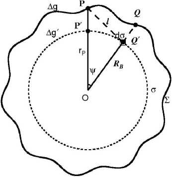
Figure 1. Bjerhammar sphere.
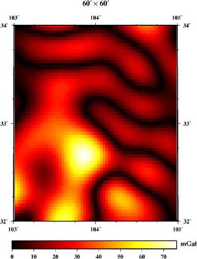
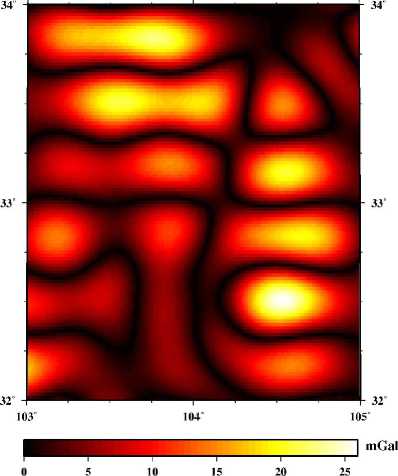
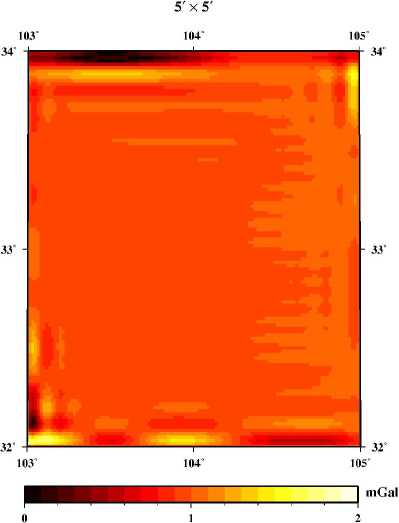
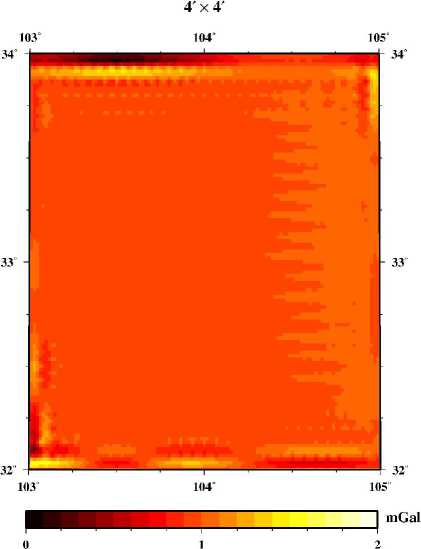
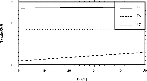
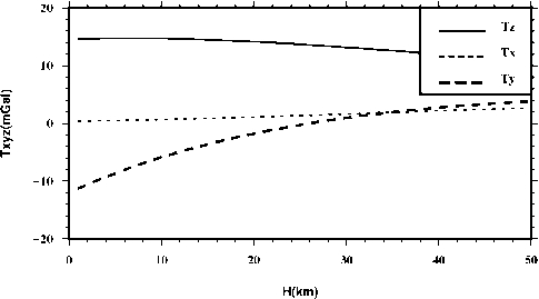
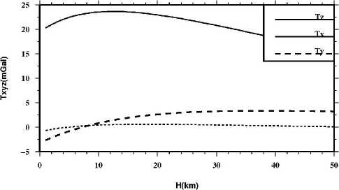
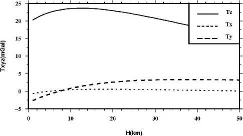
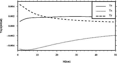
The virtual point-mass method is valid because of the Keldysh-Lavrentiev theorem [11-15]. The theorem is: If the Earth’s surface Σ is sufficiently regular (e.g. continuously differentiable), then any function f, harmonic and regular outside S and continuous outside and on S , may be uniformly approximated by functions y, harmonic and regular outside an arbitrarily given sphere CT inside the Earth, in the sense that for any given 8 >0, the relation |f-y| According to Newton’s law of gravitation, the gravitational potential at an arbitrary point P in outer space can be written as follows: Vp = A 4dCT . (1) p Cl Where f is Newton’s gravitational constant, l is the distance between P and the moving point de at the sphere C . The following formula is used to get l: l = RB + rP - 2RBrP cos у . (2) Where rP is the radius of the computation point P, у is the angle between the radius of P and de, X and ф are longitude and geocentric latitude respectively. For convenience of reference, we give the formula to obtain the angle у , as follows cos у = sin фр sin фа + cos фр cos фа cos(Xp - Xa) .(3) The range of the angle у is from 0o to 180o, so we can obtain sin у = ^/1 - cos2у . We always use the triangle functions of the angle у and the functions can be calculated through recurrence calculation of the triangle functions. To simplify the mathematics, one decomposes the Earth’s gravity field into the sum of the normal gravity field and the anomalous gravity field. The normal gravity field, a first approximation of the actual gravity field, is generated by an ellipsoid of revolution with its centre at the geocentre, called the referenced ellipsoid which of which the surface is an equipotential surface. Since the normal gravity field can be directly evaluated from simple closed formulas, the problems are converted to the determination of the disturbing potential. We assume that the anomalous potential T ' caused by virtual sphere is consistent with the one T caused by real earth. The feasibility that the outside reconcile disturbance field approximates the real field is supported by the Keldysh-Lavrentiev theorem. By assuming that the set of point masses are {mi} (i = 1,2,L , n), we can get nn T = fE mi lPi = E Mi lPi. (4) i=1 i=1 Whiei^e thie virtual messesMi = fmi , lPi is thie distance between the computation point and the moving point. We get the gravity anomaly Ag whiich is ияв! ly cis the observation dteta in geodesy and geometric, and the condition is given as follows [13] boundary дTj 2Tj' ar r = -Agj. Inserting (4) into (5), we get n Agj = E[(rj - RвC0SУji)l-3- 2jlj1]Mi . (6) i=1 This formula is the observation equation which is a linear model. Thus we can get the unknown parameters Mi according to (6). In this paper, we use least squares method to deal with the solution of observation equation. Then the anomalous potential T ' can be obtained by (4). Therefore, the gravity disturbance vector can be written as follows according to the relation between the potential and the gravity disturbance vectors: n 5r = E Mi lQ3( R в cos у - Rq) i=1 5ф = E Mi1Q3 R b(cos ФQ sin ф - sin фQ cos ф cos(A - Xq)) . i=1 5 = E MilQ3RB cosф,cos(Xi - XQ) i=1 For the point masses method, we should take the geopentation model with low degree and order into consideration. The gravitational disturbing potential can be made more manageable for many purposes if we keep in mind the fact that outside the attracting masses is a harmonic function and can therefore be expanded into a series of spherical harmonics. The gravity disturbance vector can be calculated as follows through geopentation model: fM « a n^ _* __ 5r = — E (n + 1)(_) E [ Cnm cos mX + Snm sin mX]Pnm (ф) r n=2 r fM A a —. — dP (ф) 5 =-— У (-) n> [ C cos mA + S sin mA] ф 2 v П nm nm-I - r n=2 r m=0 fM A a n-Дл — —*— 5X = - -----E (_)t m[Snm cos mX - Cnm sin mX]Pnm ф) t r cos ф n=2 r m=0 Where M is the masses of the earth, a is the equatorial radius of the earth, N is the maximum order of the geopotential model, C * and S are the model nm nm coefficients, P (ф) are the full normalized associated nm Legendre functions. Reference [16] gave some methods to deal with Legendre functions Pm (ф). In this paper, we use the WGS-84 system and a = 6378137 m. B. Formation of point-mass modle In order to analyze the point-mass model, we have a = (r - R cosy )l-3 - 2r111 which is the coefficient ji j B ji ji j ji unit of the construction matrix. The unit represents the matrix characteristic that whether the matrix is ill-posed or not. Of course, we want to obtain the stable-posed equation. Let’s assume that there are two radiuses of the virtual sphere, one is RB = 6341.555km , and the other is R = 6256.555km , while the surface is set to the mean B sphere which the radius is 6371km. We can see the variation of aji in Fig. 2. The unit aji is very small and the matrix structure can be changed by different values of polar angle у . There is purse when the angle у is close to 0. Also, we can see that the more the virtual sphere is close to the surface, the more the purse is obvious. Science the obvious purse is a good posed problem for formation of the stable matrixes, it seems that the virtual sphere’s radius should be close to the earth’s surface. In fact, when the approximated area is large and the calculated point is far from the surface, the virtual sphere discussed above can’t approximate the gravity field effectively. Therefore the importance of the selection of RB was demonstrated by Huang Mo-tao et al [14]. The variation of the distance between the virtual sphere and the earth’s surface is set to equal to the resolution of the point masses model. For example, if the model resolution is 1o x 1o, the distance is 110km. Figure 2. Variation of Uj^ with angle у . In this paper, four-tier point-mass model is constructed on the basis of EGM96 with the degree and order 36. The data of observation are calculated by EGM2008 with the degree and order 720. EGM2008 and EGM96 are the same serials model, the later is released earlier than the former. Clearly, EGM2008 is better than EGM96. The observation data are gravity anomaly which is used widely in geodesy and geodetic. There are several steps to construct the point-mass model. At first, the gravity anomaly calculated by EGM2008 with degree and order 720 minus the one got by EGM96 with degree and order 36, then we get the observation data of the first tier point masses. Therefore we can obtain the first tier point masses through the observation equation. After the first step, the gravity anomaly calculated by EGM2008 minus the one got by EGM96 and the one by the first point masses, then we get the observation data of the second tier point masses. We also use the observation equation to get the second point masses. The next step is also using the observation equation while the gravity anomaly is calculated by the subtraction of EGM2008, EGM96, the first tier point masses and the second point masses. Last, the gravity anomaly simulated by the EGM2008 minus the one got by EGM96, the one calculated by the three tier point masses, so we obtain the observation data of the forth tier point masses, like the above step, we get the forth tier point masses through the observation equation. Comparing the construction of the geopotential model [15], the formation of the point masses is very simple. So this is one of the advantages for point masses method. II. EXPERIMENTS AND RESULTS The reliable maximum order of earth gravity model is about 200 at present, as an extension, the data of gravity anomaly are calculated by EGM2008 with degree and order before 720. Four tiers of point-mass are constructed using least square method and the resolution diagram is in Fig. 3. As the first tier (A set), gravity field size is 20ox 20o, the data resolution is 1ox 1o and the range of gravity anomaly is -190.70 ~ 153.88mGal (mGal = 10-5ms-1). The second tier (B set) size is 6ox 6o while the data resolution is 20’ x 20’. The third tier (C set) size is 2ox 2o while the data resolution is 5’ x 5’, and the last tier (D set) size is 2ox 2o while the data resolution is 2’ x 2’. In order to construct a stable coefficient matrix, we set that the virtual points and the observation points are homologous coordination. Thus, the main structure of the matrix will become diagonal dominance and the stability of the matrix is guaranteed. In this paper, the gravity anomaly which is observation data is on the mean sphere, so data preprocessing is omitted. The gravity anomaly is simulated through EGM2008 with degree and order 720 and the formula can be expressed as follows: fM N a n n * Ag = ~ £ (1— ”)(-) £ [ Cmcos m^+ Sm sin m^]P,, (Ф) • r n = 2 r m = 0 Actually, we usually take the parameters f ,M as one constant. In this study, we set fM = 3.986005d+14 . ▲ -e +o+o ▲ -0+0+0 ▲ 0+0+0 * 6 ■b+o+ct Ф b+o+ct 6 "b+o+ct 6 $ ^l0^ $ Я°+^ $ Я0*^ $ ф РфО+Q. ф Р+O+Q. ф P+Q+Q. ф < -0+О+О * -0+0+0 * -0+0+0 # Figure 3. Resolution diagram for four-tier masses. The parameter RB is set to approximately equal to the resolution of observation data in the experiment. Since the true values of the disturbance gravity vector can be calculated by the EGM2008, the precision of the model is checked by the truncation error of the disturbance gravity. The center area of the approximated region is 32o~34oN and 103o ~ 105oE . The truncation errors in the radius direction are shown in Fig.4 - Fig.7. Obviously, the absolute errors of the one-tier point masses are very large, and the maximum error can reach 76mGal. However, in some areas, the absolute errors are close to 0mGal. Therefore, the approximated errors are not the system errors, and the volatility of low-frequency gravity field is sensitive with horizon distance. For two-tier point masses model in Fig.5, the errors are also large but less than the errors of the one-tier point masses. And the maximum error is no more than 27mGal. Of course, two-tier point masses model can not meet our necessary. Figure 4. Truncation errors of the one-tier point masses. Let’s see the approximated efficient of the three-tier point masses model in Fig.6, the maximum errors is less than 2mGal which is a high precision for the earth’s gravity. In addition, most of the errors are less than 1mGal. So three tier of point masses model can fit the necessary of approximation. A common sense is that high resolution of gravity field can approximate the field precisely. However, the errors of four-tier point masses model (Fig.7) with resolution 2’ x 2’ are almost equal with the errors of three-tier model with resolution 5’ x 5’, the reason is that the observation data resolution is just 15’ x 15’ which is the feature of the EGM2008 with degree and order 720. Comparing the results of the three-tier point masses and four-tier point masses, the later model has no advantage over the former one. One may argue that the point-mass model has no advantage over geopotential model. In fact, the point-mass is a method for local gravity and can be easer to approach high resolution than geopotential model. Furthermore, the point-mass model has an advantage in speed of calculation. Calculating one point’s disturbance gravity vector, four-tier point-mass model needs 0.876ms while the geopotential model takes 12.800ms at the same computer. Furthermore, the formation of geopotentail model is more complex than the construction of point masses model. 20' x 20' 103" 104" 105" Figure 5. Truncation errors of the two-tier point masses. Figure 6. Truncation errors of the three-tier point masses. A further test has also been conducted to investigate the effect of the different tiers of point-mass on the disturbance gravity vector in outside space. We compute the disturbance gravity vector on a curve line in the space and the simulation results are shown in Fig.8 - Fig.12. In these figures, the three direction vectors of δr , δϕ and δλ are shown, respectively, in the solid line (Tz), the dashed line (Tx) and the dotted line (Ty). Science the point masses method is used to approximate the local gravity field, the high frequency of the gravity field is the main content. Therefore, the range of the height on the curve is set to from 1km to 50km. Figure 7. Truncation errors of the four-tier point masses. The values of the gravity disturbing vector are from 10mGal to 20mGal. We know that the values are not large for the global disturbing gravity. And this means there is other information we do not considered into. It can be seen from these figures that the effect of goepotential model with degree and order 36 (Fig.8) is reduced slowly as the altitude increases, the maximum change of the gravity vectors is less than 3mGal. The little change means that the volatility of low-frequency gravity field is not sensitive with height. In the other hand, we must consider the effect of the low frequency of the earth’s gravity field in the high space. The effect of the first tier point masses (Fig.9) is reduced quicker than the one of the geopotential model with low order and degree (Fig.8). Comparing the gravity disturbing vector in Fig.8 with the ones in Fig.9, we can see that the volatility of the later is greater than the one of the former. It can be seen that the second tier point masses can not be ignored for the maximum gravity disturbing vectors are larger than 20mGal. It also can be clearly seen that the effect of the third tier point masses (Fig.10) can not be ignored in the low-altitude region. On the other hand, the impact of each point-mass group on gravity field could be omitted when the height reaches to a certain level. The gravity disturbing vector of the third tier point masses are about 5mGal in the low space. When the height reaches 20km, the gravity disturbing vectors are less than 2mGal. However, the topography of the test are complex, there are mountains and basins. Therefore, the information of the earth’s gravity must be abundant, and whether the effort of the third tier point masses is needed or not is determined by the limitation of truncation error. If the precision of the error is less than 5mGal, the third tier point masses must be taken into consideration. Figure 8. Disturbing gravity by EGM2008 with degree and order 36 Figure 9. Disturbing gravity by the first tier point masses We will now investigate the performance of the fourth tier point masses. The simulation results are shown in Fig.11 and the gravity disturbing vector are distinctly different with the one of Fig.10. It is obvious that the values of the disturbance gravity vectors are very small, and the maximum value is less then 0.01 mGal. The variation of the gravity unit is not large for the absolute value is too small. As a result, the information of the fourth group point-mass can be omitted in the experiment. We should like to note that, the high frequency information of earth gravity field is much more complex than the fourth group point-mass we constructed. The reason of the poor information of the fourth group pointmass is the limitation of the observation data resolution discussed above. In addition, the test proves that there is an optimal truncation error for some spectrum gravity field in the outside space. In a word, the forth tier point masses can be ignored in the simulation. However, we have to keep in mind that if the resolution of observation is more detail, the forth tier point masses should not be omitted and more tiers point masses should be constructed to approximate the gravity field efficiently. Figure 10. Disturbing gravity by the second tier point masses Figure 11. Disturbing gravity by the third tier point masses Figure 12. Disturbing gravity by the forth tier point masses III. CONCLUSIONS According to the simulation and analysis, we can get the conclusion that virtual point-mass method is a good approximation of local gravity field. An obvious advantage of point-moss model is that the calculation of the gravity units is simple. The advantage also reflects in the increasing of the calculation speed. However, the construction of point-mass model is random, a key question is how to reasonably choose the virtual sphere radius. Motivated by the success of Huang mo-tao et al. [14], the depth of the virtual sphere is approximately equal to the resolution of the point mass model in the experiments. The results of experiment show that point mass model can gradually approximate the earth’s gravity field from low to high frequency and is easer to reach high resolution than geopotential model. Furthermore, the point masses model has an advantage of calculation speed over the traditional model. In addition, the location of the point mass group and the observed values should be consistent with the coordinates, thus structure of the coefficient matrix will be stable. Finally, it should be noted that the impact of each group point masses on gravity field is closely related to the height. When reaching a certain height, some information of corresponding group point masses should be ignored to reduce the calculation. ACKNOWLEDGMENT The authors wish to thank Mr. Jiancheng Han for his constructive suggestions and valuable comments on the original manuscript. We also thank Mr. Cheng Xing, who improved manuscript in English writing. This work was supported in part by a grant from National Natural Science Foundation of China (grant No. 40637034).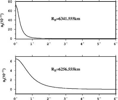

References A Study on the formation of the gravitational Model based on Point-mass Method
- Heiskanen W A, Moritz H, “Physical Geodesy,” Freeman and Company, San Francisco, 1967.
- Bjerhammar A, “A New Theory of Geodetic Gravity” Trans. Roy. Inst. Tech, No.243, 1964.
- Bjerhammar A, “Discrete physical geodesy,” Rep No.380, Dept. of Geodetic Science and Surveying, The Ohio State University, Columbus, 1987.
- Paul, E. Needham,R.E., “The Formation and Evaluation of Detailed Geopotential Models based on Point Masses,” Report No.149,Dept. of Geodetic Science and Surveying,The Ohio State University,1970.
- Sunkel. H., “The Generation of a Mass Point Model from Surface Gravity Data,” Report No.353, Dept. of Geodetic Science and Surveying, The Ohio State University, December 1983.
- Wu Xiao-ping, “Point-Mass Model of Local Gravity Field,” Acta Geodaetica et Cartographica Sinica, 1984, 13rded., vol. 4, pp. 250-258.
- Wen Han-jiang, “The Finite Element Models of Earth’s Gravity Field,” Science of Surveying and Mapping, 1993, vol. 1, pp. 41-47.
- Zhao Dong-ming, “Approximation of the Earth’s outer Gravity Field and State Estimation of Gravity Satellite,” Wuhan University, Wuhan, 2009.
- Zhang Hao, Wu Xiao-ping, Zhao Dong-ming, “A Study on Polynomial Fitting of Computing Space Disturbing Gravity with Point-Mass Model,” Science of Surveying and mapping, 2007, 32rded., vol. 4, pp. 42-45.
- Pavlis, N.k., Holmes,S.A., Kenyon,S.C., John K. F., “An Earth Gravitational Model to Degree 2160: EGM2008,” Presented at the 2008general assembly of the European Geosciences Union, Vienna, Austria, 2008, pp. 13-18.
- Li Zhao-wen, Zhang Chuan-ding, Lu Yin-long, Li Jian-wei, “Establishment of the combined Point Mass Model Considering Spectrum Characteristic,” Journal of institute of surveying and mapping, 2004, 21rded., vol. 3, pp. 166-168.
- Zhang Xiao-lin, Zhao Dong-ming, Wang Qin-bin, “Precise Determination and Approximation Analysis of Disturbing Gravity Field,” Journal of Geomatics Science and Technology, 2009, 26rded., vol. 3, pp. 212-215.
- Li Jian-cheng, Chen Jun-yong, Ning Jin-sheng, Chao Ding-bo, “The Earth’ Gravity Field Approximation Theory and China’s 2000 quasi-geoid Determination,” Wuhan university press, Wuhan, 2003.
- Huang Mo-tao, Guan Zheng “Test and Construction of Disturbing Point Masses Model,” Hydrographic Surveying and mapping, 1995, vol. 2, pp. 16-24.
- Tscherning C.C. “A Not e on the Choice of Norm when Using Collocation for the Computati on of Approximations to the Anomalous Potential,” Bull Geod, 1977, vol.55, pp. 137-147.
- Wang Jianqiang, Zhao Guoqiang, Zhu Guangbin, “Analysis of common Computing Methods of ultra-high Degree and Order fully normalized associated Legendre Function,” Journal of Geodesy and Geodynamics, 2009, 29rded., vol. 2, pp. 126-130.
