A supervised workflow for predicting lithofacies in complex and heterogeneous tight sandstone reservoirs: a data-driven approach using clustering and classification models

Machine learning (ML) is a branch of artificial intelligence (AI) that utilizes data analysis techniques such as classification, regression, and clustering to make predictions and identify patterns in large datasets. The ML approach can be classified into two groups: supervised. Supervised ML involves using input parameters and desired outputs to train a model, while ML identifies patterns without predefined outputs. In the oil and natural gas industry, machine learning has become a popular tool for solving geoscientific problems related to exploration, development, and production.Wire-line logs have become a commonly used tool for geoscientists in the oil and gas industry. With the de velopment of machine learning, various neural © Muhammad Ali, 2023

networks have been widely used in oil exploration (Antariksa et al., 2022; Song et al., 2021; Valentín et al., 2019). Chawshin et al. (2021) designed a convolutional neural network (CNN) that automatically predicted lithofacies from 2D core CT scan image slices. Alzubaidi et al. (2019) introduced a CNN-based method that used core images to predict lithology automatically, although it did not perform well in the subdivision of rock types. Zhang et al.(2021) used convolutional neural networks to identify lithofacies from core images. While these methods significantly reduced the identification time, they still required many core sample images for network training and labeling, which can be a challenge.To overcome this challenge, Zhang et al. (2021) used relatively low-cost well logs instead of core samples for lithofacies identifica- tion. This approach effectively provided a first-glance analysis of core data, although the model's generalization required improvements. Despite the limitations, machine-led applications hold great promise in the oil and natural gas industry, enabling more efficient and accurate exploration and production.

The goal of this research is to investigate how supervised classification can improve the recognition of lithological facies in a dataset. The dataset consists of complex geometrically pro-gradational sequence environments that were formed during a significant tectonic event. This event not only affects the distribution of different facies but also leads to the presence of a large volume of volcaniclastic debris, which can negatively impact the quality of the reservoir. Accurately predicting facies is important because the Lower Goru formation in the Ka-danwari gas field has the potential to produce significant amounts of natural gas. The process of facies categorization involves creating new logs, generating synthetic Gamma ray logs using machine learning regression models, and creating artificial data to fill in gaps in the dataset. The final step is to train the data samples using four different classification algorithms and select the most accurate facies classifier from the validation dataset. This study uses "ensemble learning," which combines multiple models to improve accuracy.

Area of Geology:

High Discharge Stage          Low Discharge Stage

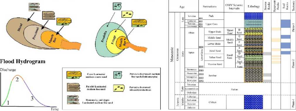
Figure 1: Sedimentology Model and lithology of the study area

Data and Methodology

This study utilized a dataset comprising wireline log measurements of six parameters, namely gamma ray ( GR ), laterolog deep resistivity ( LLD ), neutron porosity ( NPHI ), compressional wave velocity ( DT ), and bulk density ( RHOB ), as well as two petrophysical parameters estimated from the data: volume of shale and porosity. The wells sampled were located in the Lower Goru formation of the Kadanwari gas field block, which is situated in the central Indus Basin (Figure 2).

K-15 and K-14 are wells that provide facies log and facies descriptions from geological data, which we utilized as the targeted output for the machine learning (ML) algorithms in our study. The lithology of the research area is classified into six categories, and each category is identi- fied through meticulous petrophysical analysis and core investigation. Table 1contains the data and serves as a useful representation of the fluvial-based depositional system, using the facies nomenclature mentioned.

Clusters selection criteria

In the study, due to limited core facies data in the K-15 well (Figure 3), it's vital to select the right number of clusters for accurate facies representation before applying machine learning algorithms. To avoid model bias from overfitting or underfitting, two criteria are used. The Akaike Information Criterion (AIC) assesses a model's ability to predict future values based on in-sample fit, favoring lower AIC values and aiding in choosing between Holt-Winters models. The Bayesian Information

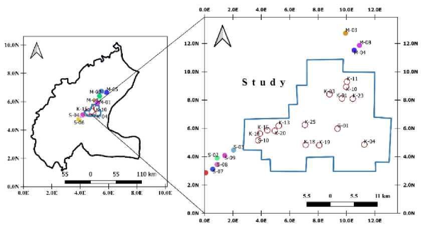
Figure 2: Geographical distribution of wells in the study area

Table 1 : facies classification of Lower Goru

Facies	Description
Sh	Shale to silty Shale (Shelf deposits)
Slst	Siltstone to silty-shaly sandstone (prodelta shales with turbiditic layers)
Css	Low-porosity, low permeability cemented sandstone (very distal mouth bar fringe)
Lss	Low-medium porosity, low permeability sideritic/chamositic sandstone (shoreface to distal mouth bar)
Ss	High-porosity, high permeability sandstone (mouth bar)
Hs	Highly chamosite/siderite affected lithologies (chamositized mouth bar)

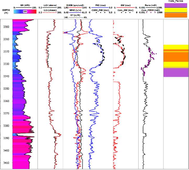
Figure 3: Visualize core facies data in the small section of well K-15

Criterion (BIC) balances model complexity and fit, with lower values indicating a better fit. The study provides equations to compute AIC and BIC values for model selection, ensuring the optimal cluster number is chosen for machine learning in cases of limited core facies data in the K-15 well.

One-Class Support Vector Machine (SVM):

Support Vector Machine (SVM) is a supervised machine learning algorithm used for classification and regression tasks(Vapnik, 1995). It finds the optimal hyperplane that best separates data points into different classes while maximizing the margin between them. SVM is effective in handling high-dimensional data and can also be used in non-linear scenarios by employing kernel functions.

Neural Network:

A neural network is a computational model inspired by the structure and function of the human brain. It consists of interconnected nodes, or artificial neurons, organized in layers, which process and transform input data to produce output. Neural networks are used in various machine learning and deep learning tasks, such as image recognition, natural language processing, and more, by learning complex patterns and relationships within data (Guresen & Kayakutlu, 2011; Haykin, 2011).

Random Forest:

A random forest is an ensemble machine learning method that combines multiple decision trees to make more accurate predictions or classifications (Akkurt et al., 2018). It mitigates overfitting and increases the model's robustness by aggregating the results of individual trees, often resulting in improved performance and generalization.

Data Split and Cross-Validation:

In machine learning, data partitioning is critical to ensure effective model evaluation on new data. Typically, data is split into a training set for model training and a testing set for final evaluation (Alghazal & Krinis, 2021). For small datasets, the risk of overfitting to the training data is a concern. To address this, cross-validation is used. It involves breaking the training set into multiple folds. The model is evaluated on each fold while being trained on the others, reducing overfitting. After cross-validation, the model with the best score is selected and used to predict the testing set for the final evaluation ( Figure 4).

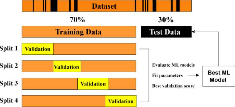
Figure 4: The visual representation of the dataset is divided into two sets. The first one is training and the second one is testing the dataset for the machine learning model

Feature Selection:

Feature selection is a crucial step in reducing dataset complexity by removing irrelevant features. It benefits machine learning in several ways (Ali et al., 2021; Guyon & Elisseeff, 2003; Li et al., 2017), including simplifying models, saving time and costs, reducing overfitting risk, and mitigating data dimensionality issues. This study employed two feature selection methods: univariate and Pearson's Correlation (r). Univariate selection individually tests each feature's relationship with the target variable. Pearson's Correlation measures the strength of linear relationships between pairs of variables, with values ranging from -1 to +1, where 0 implies no correlation, negative values indicate a negative correlation, and positive values indicate a positive correlation.

Criteria for verifying model performance:

Precision =

True positive

True positive + False positive

Recall =

True positive

True positive + False negative

1= 1 (    ¹     .    ¹ A            (3)

F 1   2 Precision Recall

Result and discussion:

This section has multiple parts. First, we determine the cluster count in the study area using our novel algorithm from previous section. Then, we reduce dataset complexity with feature selection techniques, normalizing features for better machine learning convergence. In the third part, we compare lithology identification results for each model. Next, we evaluate algorithm efficiency. Finally, we apply the final model to predict well facies and check the prediction accuracy based on synchronization measures for synthetic logs.

Cluster Analysis:

The pivotal step in clustering analysis is visually assessing the two-information criteria plot to pinpoint the ideal number of clusters. This is done by identifying inflection points in the Euclidean distance plot, which indicate that further clusters do not significantly enhance data characterization. In Figure 5, the AIC/BIC curves level off at six clusters, signifying an effective model for describing the study area well logs' facies.

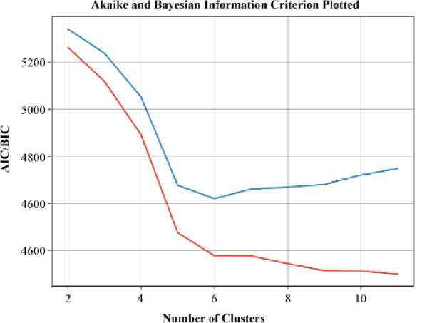
Figure 5. Determining the optimal number of clusters using the two-information criteria plot

Feature selection:

Before model training, selecting the most relevant feature with a strong target correlation is vital. In this study, eight logging curves were chosen, excluding TVD, LLM, and LLS. Results in Figure 6 show Gamma (GR) had the highest impact (Influence Factor 36.21), followed by Deep Resistivity (LLD, 16.04), Com-pressional Sonic (DT, 13.17), Density (RHOB, 9.85), and Neutron (NPHI, 7.70). Photoelectric factor (PEF), Spontaneous potential (SP), and Caliper (CAL) were least impactful (Influence Factors ≤6). Thus, the top four inputs (GR, LLD,

DT, RHOB) are most crucial for facies evaluation.

After estimating the cluster count from the two-information criteria plot, core facies and selected logs are added to the training data, leaving out the blind/testing well. One well's data is reserved for algorithm evaluation. Figure 7 shows the facies distribution in the training dataset, highlighting the underrepresentation of High-porosity, high-permeability sandstone (Ss) facies compared to others. To enhance prediction models, more Ss facies samples should be obtained.

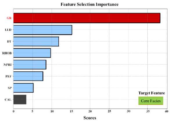
Figure 6. Feature importance scores of input features versus core facies

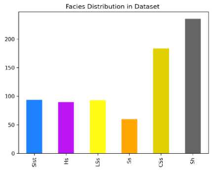
Figure 7. Facies (class) distribution of the training data

Facies predictions utilizing ML models and comparison:

In our study, we evaluated ML models for facies prediction. Initially, default models were tested on the training dataset using confusion matrices to measure accuracy. This tool helps assess model effectiveness and estimate misclassification losses. For identification performance, we used metrics like precision, recall, and F1-score. Figure 8 displays model performance. GPC excelled, followed by SVM and ANN, while RF performed the poorest. In lithology identification, ensemble models outperformed RF, with GPC leading. Different models had varying success with different facies types. While all performed well with certain facies, RF struggled with Ss. GPC performed the best overall, slightly outperforming ANN. SVM was weaker in identifying Hs, LSs, CSs, and Sh compared to ANN, highlighting ensemble models' advantage with non-uniform facies. Figure 8 shows confusion matrices, illustrating how predicted facies compare to actual facies for each lithofacies. For instance, in the GPC model's matrix, common misclassifications included 3% of samples as Hs, CSs, and Sh, and 3% of CSs samples as Sh. These errors result from overlapping logging features in the misclassified lithofacies. Nevertheless, the GPC model outperformed others, achieving high lithofacies prediction accuracy, as shown in Figure 8.

Confusion Matrix Based on SVM Model
Prediction	Slst	Hs	LSs	Ss	CSs	Sh	Total
Sisi	Q	5		0	3	И	21
Hi		16		0		0	19
LSs	0	0	18	0	0	0	18
Ss	0	1)	10	7	0	0	17
CSs	0		0	0	37	0	38
Sh	0	D	0	0	6	33	39
Table: Prediction Accuracy Score
Precision	(1.67	0.73	0.5*	1	0.82	0.75	0,76
Kerall	0.1	0.84		0.41	0.97	0.85	0.74
Fl	(117	0.78	0.73	0 58	0 89	0.8	0.7

Confusion Matrix Bawd on ANN Model
Prediction	Slst	Hs	LSs	Ss	CSs	ShT	Talal
Slst	9	9	0	0	0	3	21
Hs	1	16	2	0	0	0	19
LSs	0	0	16	2	0	0	18
Ss	0	0	0	17	0	0	17
CSs	0	1	0	0	35	2	38
Sh	1	0	0	0	3	35	39
Table: Prediction Accuracy Score
Precision	0.82	0.62	0.89	0.89	0.92	0.88	0.85
Recall	0.43	0.84	0.89	1	0.92	0.9	0.84
Fl	0.56	0.71	0.89	0.94	0.92	0.89	0.84

Confusion Matrix Based mi GPC Model
Prediction	Slst	Hs	LSs	Ss	CSs	Sh	Total
SU	16	3	0	0	1	1	21
Ik		16	2	0	0	0	19
LSs	0	0	17	1	0	0	IS
Ss	0	0	0	17	0	0	17
CSs	0		0	0	36	1	38
Sh	0	0	0	0	3	36	39
Table: Prediction Accuracy Score
Precision	0.94	0.8	0.89	0.94	0.9	0.95	0.91
Recall	0 76	084	0 94	1	095	0 92	0.91
Fl	0.84	0.82	0.92	0.97	0.92	0.94	0.91

Confuskm Matrix Based on RF Model
Prediction	Slst	Hs	I.Ss	Ss	CSs	Sh	Total
Sisi	16	3	0	0	0	2	21
Hs	5	12		0	0	0	19
LSs	0	0	18	0	1)	и	IS
Ss	0	0	17	0	1)	0	17
CSs	1		4	0	32	0	38
Sh	0	0	0	0	9	30	39
Table: Prediction Accuracy Score
Precision	0.73	0.75	0.44	0	0.78	0.94	0.68
Recall	0.76	0.63	1	0	0.84	0.77	0.7]
Fl	0.74	0.69	0.61	0	0.81	0.85	0.68

Figure 8. Confusion Matrix of SVM, ANN, GPC, and RF facies prediction outcomes and Specific facies are identified by their labels and explained in the table

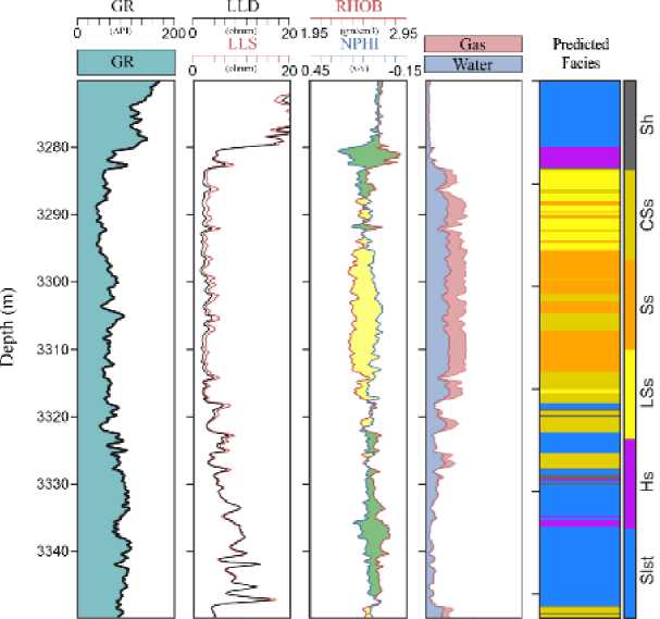
Figure 9. The prediction results of final models for K-14 well (blind well)

In the last step, we used the GPC model to predict lithofacies in the testing dataset and checked the accuracy based on synchronization measures for synthetic logs. Utilizing core data from K-15 wells, we extended facies predictions to wells without core data. Figure 9 shows the facies distribution in a blind well using the GPC model. The first four plots display measured logs with depth (in meters), and the last track shows the predicted facies track by GPC.

To assess facies prediction accuracy without ground truth data in Figure 9 (blind well K-14), a novel technique was used. It confirmed predictions by leveraging elastic parameters such as acoustic impedance and velocity ratio, which are linked to reservoir quality and lithofacies. An acoustic impedance vs velocity ratio cross plot was generated for the blind well based on predicted lithofacies, producing 2D probability density functions (PDFs) (Figure 10a and b). These PDFs represent each sample's similarity to data points within its cluster and dissimilarity to those outside its cluster. They were then used as input with depth in a neural network to predict synthetic gamma-ray log responses (Figure 10c). Since the gamma-ray log is crucial for rock type differentiation, its prediction accuracy was evaluated using synchronization measures. Figure 10d compares actual gamma logs (GR)

with predicted synthetic logs (Syn_GR) from the neural network, showing visually satisfactory results with nearly identical average log trends. Cross plots between measured GR and predicted Syn_GR from the machine learning algorithm for blind wells are displayed in Figure 10e. These plots quantitatively measure the algorithm's predictive ability, yielding a satisfactory R2 value of 0.978.

After predicting lithofacies using well log data, the inverted acoustic impedance and Vp/Vs volumes were used to classify the predicted lithofacies. This information was then used to construct a facies prediction volume. The inverted facies volume is strongly correlated with the predicted lithofacies at the well locations (Figure 11a). To ensure quality control, the Vp log was compared to the Vp modeled from the predicted porosity volume generated from inversion utilizing the facies model, and the Vp modeled from the original porosity log. The modeled Vp calculated based on the porosity log correlates well with the Vp log, and the predicted Vp from inversion shows good correlation with the measured log (Figure 11b), especially in the upper section of the well where the reservoir facies are present. Overall, the model performs very well and effectively differentiates the rock types.

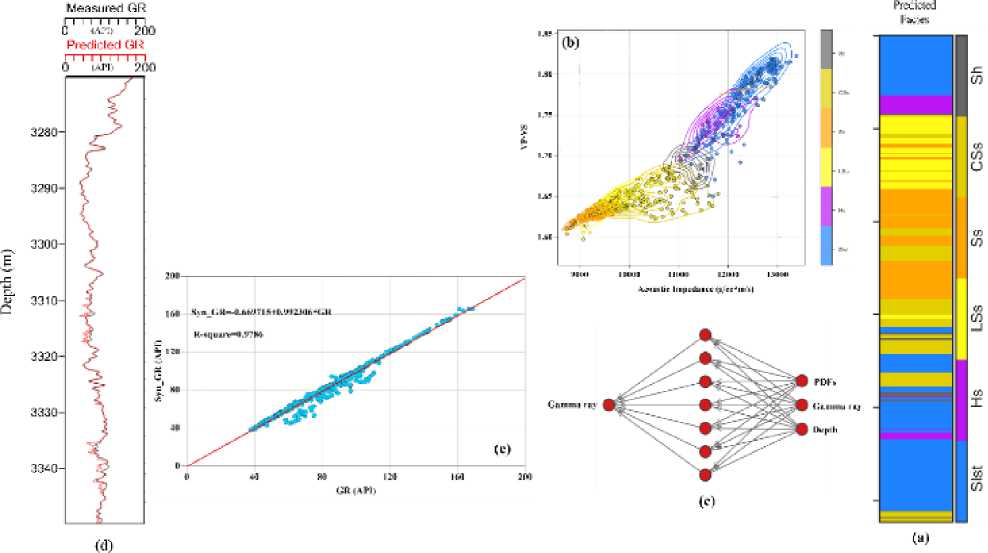
Figure 10. Result of the blind well (a) predicted lithofacies (b) based on lithofacies extract PDFs (c) utilized neural network to predicted synthetic log (d) actual and predicted gamma-ray log response comparison trend (e) check the prediction accuracy result by the least square method

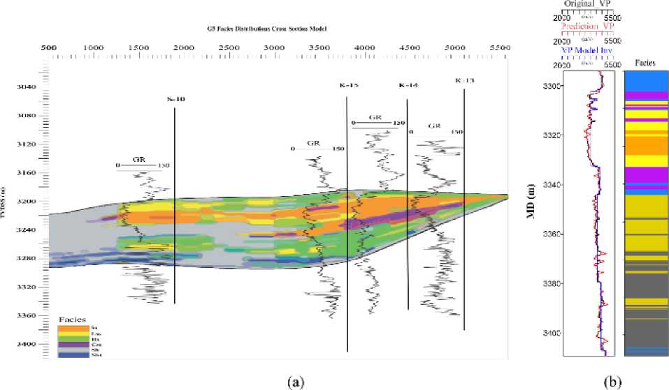
Figure 11. Displays two panels: (a) the facies prediction volume generated by classifying the predicted lithofacies using the inverted acoustic impedance and Vp/Vs volumes, and (b) a comparison of the original Vp log, Vp predicted from the facies model applied on the original porosity log, and modeled Vp obtained from the predicted porosity volume derived from inversion using the facies model

Conclusion:

A new workflow for lithofacies prediction using supervised machine learning algorithms was developed. The novel two-information criteria clustering approach generated facies that were strictly data-driven. Four supervised machine learning classifiers were employed, with the GPC model achieving the highest identification performance. The GPC model was used to predict lithofacies in the testing dataset and the accuracy of facies similarity was assessed by synchronization measures to predict synthetic logs. A 2D probability density function was generated from an acoustic impedance vs velocity ratio cross plot of a blind well based on the predicted lithofacies. This was used as input with depth in a neural network to predict synthetic gamma-ray log response. The results obtained from the neural network were visually satisfactory, with a high correlation between the measured GR and predicted Syn_GR from the machine learning algorithm at blind wells (R2 of 0.978). Finally, the predicted lithofacies were used to create a facies prediction volume, which correlated well with the predicted lithofacies classification. The workflow provides consistent, reliable, and efficient results, saving time and effort in data processing and interpretation.