About Lyapunov exponents identification for systems with periodic coefficients

Author: Nikolay Karabutov
Journal: International Journal of Intelligent Systems and Applications @ijisa
Article in issue: 11 vol.10, 2018.
Free access
Lyapunov exponents (LE) identification prob-lem of dynamic systems with periodic coefficients is con-sidered under uncertainty. LE identification is based on the analysis of framework special class describing dy-namics of their change. Upper bound for the smallest LE and mobility limit for the large LE are obtained and the indicator set of the system is determined. The graphics criteria based on the analysis of framework special class features are proposed for an adequacy estimation of obtained LE estimations. The histogram method is applied to check for obtained estimation set. We show that the dynamic system can have the LE set.
Dynamic systems with periodic coeffi-cients, Lyapunov exponents, framework, histogram
Short address: https://sciup.org/15016539
IDR: 15016539 | DOI: 10.5815/ijisa.2018.11.01
Text of the scientific article About Lyapunov exponents identification for systems with periodic coefficients
Published Online November 2018 in MECS
Lyapunov exponents widely apply to the analysis of dynamic system qualitative behavior. They allow estimating trajectory behavior of various objects in physics [1], medicine [2-4], economy [5], astronomy [6]. LE determine on the basis of time series analysis most often. Many authors suppose that the a priori information is known about system structure. [7] contains the review of large LE calculation for various classes of systems. Lyapunov exponents estimation algorithm for an unknown dynamic system is proposed in [8]. It allows calculating all LE and is based on the application of networks with the multidimensional prediction. The basis of the network is monotonic sigmoid functions. The task solution is based on parameter selection of functions approximating a time series on the square criteria.
Various algorithms use for calculation of the large LE for time-varying systems on experimental data. Application of these algorithms is based on Takens theorem [9]. Takens showed that the phase portrait (attractor) of a system can be recovered (reconstructed) on the basis of one time series (experimental data). Therefore, the theorem is the basis for calculation of various indicator dynamic system. Takens theorem is a basis for the LE estimation. Wolf [10] and Rosenstein, Benettin [11] methods apply to the definition of the large LE. Many authors generalize and develop these methods. In [12], algorithms are proposed for the calculation of the large (first) Lyapunov exponent based on logarithm and interpolation of a time series, and also a method of logarithm allocation. The application of the interpolation algorithm gives best results for time-varying systems. The model having the form of the exponent and the sinusoid with phase shift is proposed for compensation of a nonstationary component in a time series. Such approach allows eliminating a non-stationary component from the time series. This procedure is not applicable for time-varying system LE identification as it is removed with a layer of valuable information. Notice that implementation of Rosenstein method represents the labor-consuming procedure associated with choice and specification of system parameters. The neural network algorithm is proposed in [13] for the estimation of the largest LE. It is based on the application of multilayer perceptron.
Two main methods exist for Lyapunov exponents estimation on the time series [14]. The application of these methods is based on previously a recovered attractor in a phase space of some dimension with the help of Takens theorem. The first method [10] determines by two close trajectories in the recovered phase space and traces their behavior on some time interval (Benettin's algorithm [ 15]). The estimation of the LE spectrum is obtained to the scheme coinciding with LE procedure calculation on an initial system of equations and equations in variations. The relative simplicity is the advantage of this method. The shortcoming of this method is the difficulty of all spectrum Lyapunov exponent identification as the determining role by consideration of two close trajectories is played with the large LE. The second method [16, 17] is based on the use of Jacobin as LE is possible to determine by as Jacobi matrix eigenvalues for a system which generated the considered realization. The advantage of this method is the possibility of non-negative Lyapunov exponents spectrum estimation on short implementation, and the shortcoming is high sensitivity to noise and errors for which reduction various methods and algorithms are used.
Application Takens theorem which is widely used for system State reconstruction in the form of frameworks depends on features of the time series [18]. Naturally, it influences on the efficiency of criteria applied to the orderliness estimation of the system (an attractor). Implementation complexity of LE identification methods can be explained with features of the time series.
So, various method modifications of Rosenstein,
Benettin, Wolf and Takens theorem are widely applied to Lyapunov exponents identification of stationary systems. Properties of the time series describing change of system variables have significant effect on the accuracy of obtained LE estimations. Various modifications which included the available a priori information are developed for application simplification of specified methods. These approaches are applied to LE estimation of time-varying systems. As a rule, the considered methods allow finding the high (first, large) Lyapunov index. The overwhelming number of publications is devoted to the analysis of systems in which there can be chaos. Time-varying systems have the specifics [19]. In particular, they may contain Lyapunov exponents set. The further modification is required for the approaches and methods considered above for LE estimation. Criteria and procedures for verification of obtained decisions are proposed not always. In [20] the approach to identification of Lyapunov exponents based on the analysis of frameworks special class is proposed. Frameworks describe LE change dynamics of stationary systems under uncertainty. They do not demand the application of the procedures and methods considered above. Below generalization is given this approach on a class of periodic systems.
The paper has the following structure. The problem statement is given in section II. The method of system general solution obtaining which is the basis for identification of LE is described in section III. The static model is proposed for determine of system general solution and the question its an identifiability (section IV) is considered. Section V contains formulas for calculation of characteristic indicators. The system coefficient of structural properties which is a basis for the design of frameworks considered further is proposed. Section VI contains bases almost periodic functions to Bohr and the concept an -almost periodic function in Bohr sense is introduced. Framework design method for the LE estimation is stated in section VII. Further frameworks are applied to the estimation of system order and Lyapunov exponents set (sections VIII, IX). Modeling results are presented in section X.
-
II. R elated W orks
We apply a standard formula to LE deriving [9, 14, 19]. Obtained arrays for LE are the basis for the design of frameworks reflecting LE change dynamics in special structural space. We apply an approach and a method proposed in [20]. The structural approach allows determining by a parameter number for LE which are obtained theoretically in [19]. The criteria proposed for LE set select are based on the idea of paper [20].
-
III. P roblem S tatement
Consider the linear dynamic system
X = A( t) X + BU, Y = CX + WVU, where X e Rm is state vector, U e Rk , Y e Rn are input and output, Wn e Rnxk, C e Rm , A(t) e Rmxm, B e Rmk .
Let the matrix A ( t ) satisfy conditions.
A1. A ( t ) is a continuous Frobenius matrix and limited.
|| A(t )|| < a a (2)
where a > 0, IHI is norm of a matrix.
A2. A ( t ) is almost periodic [19], i.e. the subsequence which is uniformly convergent on all axis to some almost periodic matrix A ( t ) can be chosen from any sequence [19]
AZ (t) = Az (t-т).(3)
A3. A ( t ) is Hurwitz matrix for almost all t > 0 .
Experimental information for (1) has the form
Io ={Y(t), U(t), t e J = [10,ti]} .(4)
Write the solution of the system (1) as
X (t) = X (t0, U, t)(5)
where X is the operator who is determined by matrixes A , B .
Obtain from (5) the solution of system (1) at X 0 = X (t 0 )
X ( t ) = X g ( t ) + X q ( t ), (6)
where Xq ( t ) is a particular solution (1) with U e Io , Xg ( t ) is a general solution (1) with U ( t ) = 0 at the unknown X o e Io.
Let X ( X , t ) is a general solution of system (1) with X 0 = X 0 Y 0 ) e I o .
Task: determine by decision estimations
X g ( t ) = X g ( X q , X 0 , t )
on the set I and make the decision on eigenvalues spectrum and the order of system (1).
-
IV. E stimation X ( t )
Apply operation { X(t ) } \ { Xq (t ) } and create the set { Xg ( t ) } for LE estimation.
We will state solution method of the task [20] on the example of second order system (1) with one input and an output. Wv = 0 . Introduce designations: y = Y , u = U .
Let D ( to ) , Du ( to ) are frequency spectrum u , y , | y(t )| < да , | u(t )| <да . As the matrix A(t ) satisfies the A3 condition obtain Dy ( to ) ^ Du ( to ) , i.e. the system (1) is time-varying. The proposed approach to the design of a model eliminates this delay.
Present I as
Io = Iq (Jq )ui g (Jg), where Jq U Jg = J c R ; I q , I g are sets containing the information about X and X .
Determine by particular solution estimation of the system (1) on the set I q ( Jq ). As x = y , y g R apply variable y differentiation operation to obtaining the component x2 = x vector X g R 2. Designate x2 = y .
Statement 1 [20]. Model
X q ( t ) = A q W ( t ) V t g J q (7)
is applicable for the identification X ( t ) on the set I q where A g R 2x2 is the parameter matrix of the model, W = [ u u T .
Model (7) properties depend on the choice of the interval Jq c J . The model (7) is applicable also to the case m > 2 .
Determine by the estimation of the particular solution X ˆ ( t ) of the system (1) using the model (7) on the set I g . Next obtain the estimation of general solution
/X
Xg (t) = X(t) - XTq (t) Vt g Jg, where Xg (t) = [yg (t) yg (t)] .
The proposed approach is generalized to the multidimensional case. Further we consider the system (1) with one input u and one output y . We suppose that the system (1) is identified. Perform this condition check on the basis of the approach proposed in [20].
-
V. LE. S ystem C oefficient of S tructural P roperties
Apply Lyapunov exponents [19] to the estimation of system (1) properties. LE for a real function h(t) determine as ln h(t)
X [ h ] = hm I1'. (8)
t ^” t is lim upper limit. t 2да
LE x ( i = 1, m ) of stationary system (1) nonzero solution coincides with real parts of matrix A eigenvalues X .
Let the estimation of general solution Xg ( t ) V t g Jg be known for the system (1) and condition A3 is satisfied. Apply (8) to y ˆ g ( t )
ln y ˆ ( t )
x [ yg ] = lim-------, (9)
L g t ^ t t where t g Jg is the upper bound t on an interval Jg c J.
-
(9) there is large LE. If the limit (8) exists, that x [ y g ] is matrix A maximum eigenvalue estimation. Therefore, X [ y g ] is the stability degree of the system (1). If m = 2 the obtain for y ˆ
ln y ˆ g
-
X [ yg ] = lim
Also, the indicator ln h(t)
П h ] = lim——-,(11)
t i« is applied where lim is the bottom limit. It is the Perron bottom index [19, 20].
The idea of Lyapunov exponents application in identification problems is presented in [20]. The proposed approach is based on the analysis of structural properties coefficient (CSP) [20]. Below development of this approach is given. Show at first to an association between CSP and LE.
Introduce the indicator for the system (1)
^ ( y g ) = P g = ln| y g (t )| V t G J g c Jg , (12)
where Jg = [ t 0, t ] determine on the basis of (9).
Consider a system with the input t and the output p ( y g) . Then CSP for the estimation of system structural properties has the form
p ( y8 ( t ) )
k s ( t , p ) = V g 7 . (13)
ks ( t , p ) is the main variable for indicator x [ y g ] calculation on the interval J .
So, interdependence between LE x [.yg ] and the coefficient of structural properties ks (t, p^ is showed on the informational set Ip = {p(yg (t)), t e Jg,}.
Consider the set
I g ( y g , t ) = { y g ( t ), t e Jg } = I Jg \ { y g (t ) t e Jg } , (14)
which data about the change of the variable y ˆ contains on the interval J .
We suppose that the system (1) is stable, i.e. Re( ^ ( t )) < 0, i = 1, m for V t > 0 where ^ ( t ) ea (A) is i -th state matrix eigenvalue.
Problem: estimate Lyapunov exponents and the order of the system (1) on the basis of sets I , I analysis.
As the set (14) is formed on the basis of the model (7), the obtained estimation y g will contain error г . Therefore, the function y ˆ ( t ) will be almost "periodic".
-
VI. A lmost P eriodic F unctions to B ohr
Consider a class of almost periodic functions to Bohr.
Definition 1 [ 21 ] . The numerical set E = { ^ } is called relatively dense on the real axis -да< x <да if such number 1 > 0 exists that each segment a < x < a + 1 of length l contains at least one element of our set, i.e. at any a we have
[ a , a + 1 ] nE # 0.
Definition 2 [ 21 ] . The number T = Tf ( 6 ) is called almost the function f ( x ) period accurate within 6 (or 6 -almost the period or 6 -shift) if inequality
I f ( x + T f ) - f ( x )| < 6 , 6 > 0 (15)
fairly for any x e ( -да , да ) .
Definition 3 [ 21 ] . A function f ( x ) e ( -да , да ) is called almost periodic in Bohr sense ( BF -function) if relatively dense almost T set of the function f ( x ) exists accurate within 6 , i.e. such positive number 1 = 1 ( 6 ) exists that any segment [ a , a + 1 ] contains, at least, one number T- for which it is fair
| f ( x + T ) - f ( x )| < 6 for x e ( -да , да ) .
where 6 is any positive number.
Function yˆ (t) belongs to exponential-sinusoidal function class. Therefore, the condition (15) cannot be satisfied. Provide the belonging yˆ (t) to BF -functions.
Perform the following operations.
Consider some point t e R and its neighbourhood Ot .
Determine the average value yg (t) for Vt e Ot a = уg,Ot \^у 1,
Nt i where Nt is the point quantity on Ot, t e Ot is the current coverage of the interval Ot with a step т .
For t e R belonging to the neighbourhood Ot+T obtain yˆg
П = yg,Ot+Tyg V ^yi , g Nt+T- i yg
Definition 4. The function y g ( t ) e ( -да , да ) is called almost periodic in Bohr sense ( BF -function) if relatively dense almost T set of the function y ˆ ( t ) exists accurate within 6 , i.e. such positive number 1 = 1 ( 6 ) exists that any segment [ a , a + 1 ] contains, at least, one number Tf for which it is fair
У g ( t + Tf )
П
y ˆ g ( t )
a
< 6 for t e [0, да ) .
-
VII. F rameworks for LE E stimation
State to the approach to the LE estimation based on the analysis of frameworks proposed in [20].
Consider sets
I k s = { ks ( t , P ( yg (t ) ) ) , t e Jg } ,
I k s = { k s ( t , P ( Уg (t ) ) ) , t e J g } .
Determine on Ik , Ik, mapping Sk c I^. x I , . The s ss ss, p ss ss framework S describing LE change dynamics. Consider on the set I^, the function
A k ‘ ( t ) = ks ( t , p ( yg(t + т ) ) ) - ks ( t , p ( :yg ( t ) ) ) (16)
describing the change of the first difference ks ( t , p ( y g ( t )), where т > 0 .
Form the set IM , = { a ks ( t , p ( y g ( t ) ) ) , t e J g } and consider the framework SK^k, defined on I^ x IM , . Consider the mapping
LSK A k ‘ , , ^ I k . , - B ( I A k s , , ) , (17)
for the framework SK^k, where B (I^, )c {-1;1}. De fine by elements of the binary set B (IM, ) as
1 if A k ‘ ( t ) > 0, b ( t ) = ,
[-1 if Ak‘ (t) < 0, t g Jg.
Remark 1. The border of the limit superior to (9) is chosen on basis of the change S .
Remark 2. Values range choice of the function b ( t ) is defined by the convenience of its graphic analysis. b ( t ) is possible to define on the binary set {0; 1}.
The stated approach was proposed for a class of stationary systems. Some modification has required this approach for an -almost periodic systems. In particular, the framework LSK effectively works in the analysis v s, p of stationary systems. LSK is inefficient for periodic v s, p systems as the function b(t) reflects all changes in the framework SK .
Ak s , p
-
VIII. S ystem O rder E stimation
All results presented further belong to the system (1) with Frobenius matrix y g R , Wv = 0 , U = u , u g R . We consider that the matrix A satisfies A1-A3 conditions.
Propose a criterion for the estimate of the system order. It is based on the modification the theorem 1 [20] to consider specifics of the considered system.
Consider the framework defined on I^ x IM, and de scribed by function fk (t) : ks ^ Aks . The function f(t) is BF -function. Therefore, f(t) contains areas D which have sharply changing amplitude.
Definition 5. The area D of the function f is called an -area on the interval Jsk = [ t , t + T ] changes t if it corresponds to the change BF -function k ( t ) on this interval.
Theorem 1. Let the system (1) satisfy conditions A1-A3. Then the system (1) have an order m if the function f ( t ) contains not fewer m areas D on the interval [ t 0 , t ‘ J g ( t * ^ ) .
Proof of Theorem 1. Consider the case of simple real roots. The system (1) is stable. Let system eigenvalues of the system (1) be located in decreasing order
4 > ^ > ...> ^ . \(t) (i = 1,m) is the periodic func tion. The function exp (^ (t)t) g yg is an -almost periodic on some subinterval J^ c J . exp (^ (t)t) corresponds to LE x belonging to the lineal L(t) , and x corresponds to the area Disk on the framework SK^k, . The area Di is congruent in system (1) decision space to the lineal Lm-i (t) (see definition [19]). The transition between lineal can be performed m -1 time. The function p(yg (t)) depends from yg (t), therefore, each such transition gives to the change of framework SK proper-v s, p ties.
Remark 3. As matrix A eigenvalues \ ( t ) are periodic functions of time, a lineals L i ( t ) and L + 1 ( t ) can be intersected. This case can lead to an infinite LE spectrum. This feature is noted in [19].
Remark 4. If frequency spectra of lineal Li ( t ) and L + 1 ( t ) are intersected, then we have instead of the pyramid [19] corresponding to a step set of lineal
0 = L 0 (t ) c L l (t ) c...c L n (t ) = L1 ( t )
the pyramid with almost smooth sides. Such representation influences on obtained Lyapunov exponents spectrum.
-
IX. S tructural A pproach to LE E stimation
Below we develop an approach which does not demand the set I processing to the identification of Lyapunov exponents. It is stated in [20] and based on the analysis of frameworks properties proposed in section VI. The approach is based on the analysis of system framework S change in a special space.
It is known [20] that system characteristic indicators influence on a change S . Consider frameworks S and
SK i ( i > 1) an example of a framework S .
k s , p
We introduce the framework SK i which is defined on ks, p the set Ik x Iand SK^k, where i designates i -th de rivative yˆ (t),
I k. = { ks ( t , p ( y gi ) ( t ) ) ) , t G J g } . (18)
The framework SK i as shown in [20] reflects LE ks, p change. Indicators x [.yg ] correspond to local minima
SKv . X correspond to a global minimum, a x ks, p correspond to a maximum of the function describing the change SK i .
k s , P
Theorem 2 [20]. If the system (1) is stable and contains simple eigenvalues, then frameworks SK t , i = 1, m ks, P contain the information on Lyapunov exponents.
The local minima location on SK i coincides with arks, P eas Dsk of the framework SK^k, . The analysis Disk gives the set M containing LE estimations of the sys tem (1). The cardinal number M cannot coincide with LE
Lyapunov exponent’s number of the system. M char acterizes an available set of system (1) lineales.
Perform the choice of time t in (10) on the basis framework SK^k, change analysis.
Remark 5. The framework SK i where i > 1 can be
Л ks, P applied decision-making on LE.
The proposed approach gives the estimation of the smallest Lyapunov exponent n [yg ] • It is the difference between this approach and procedures proposed in the literature. If the framework SK^k, contains single abrupt change of the value, then it is a sign that SK i contained ks, P the estimation nm [']. As |nm t’H > Xi ['ll where i = 1, m -1, n ['] designate as к and call the upper bound of the smallest LE. Explain this fact that the corresponding lineal Lm (t) has the minimum definitional domain. Function yg (t) on Lm (t) is not an -almost periodic, so its parameters a,n quickly decreases. Therefore, the condition (15) is not satisfied. Therefore lineal Lm (t) contains only one value which corresponds к . So, fairly
Statement 2. Let the system (1) satisfy conditions A1-A3 and the framework SK i contains a point M in which
Лks, P value sharply changes. Then the global minimum corresponds to the point M on the framework SK i and the ks, P global minimum value is the upper bound к of the smallest n [yg ] .
Remark 6. As the decision is to accept on the basis of several frameworks SK i ( i > 1 ) choose the upper ks, P bound from к,i and designate it as к .
The set M is formed on the basis of minimum LE
SK i analysis and the remark 5.
k s , P
Consider the definition problem of the domain which belong the set M . Explain it with the fact that the set M can be big (see the remark 3). Find an admissible domain for M and the number defining mobility of the highest Lyapunov exponent. This domain is limited to the indicator к from below. Determination of the specified parameters is realized on the interval [ 0, t ] where t is chosen according to (9). Realize variation domain x choice on the basis of the framework SK i analysis.
Л k s , P
The area D^ c SKt is the existence x indicator. The s, P fragment V 1i on the framework SK i which changes ks,P ks, P on the interval J 1i corresponds to the area D1 . There- ks, p fore, x G J1 i . Then the admissible mobility boundary ks, P of the higher indicator x is determined as
X 1 ^ sup J 1 . (19)
k s , P
The inequality (19) gives to the admissible boundary (boundary of mobility on [19]) the change x under uncertainty. Areas of mobility for x ( i > 1) are determined similarly.
Consider criteria for the estimation of set M ele-LE ments and (19). The concept of the adequacy accepted in parametrical identification theory in this case is inapplicable. As shown in section I, the publications majority is devoted to the calculation of Lyapunov exponents. Questions of the quality check of obtained estimations were not considered. Such theoretical indicators as durability attainability do not give in to validate under uncertainty. Further, the method is offered for verify so-called / -adequacy of obtained LE estimations. It is based on the analysis of frameworks proposed above.
Consider the framework S described by the func-yˆg,yg tion f , : y ^ y in space R =(y , y ). As the sys-y, y gg y g g tem (1) satisfies A1-A3 conditions, S contains areas yˆg,yg which reflect an -almost periodic behavior of the system.
Consider frameworks SL i and SL i which are deA ks, P ks, P scribed by functions fL. : У ^ ks, p , fL, : У ^s, p . (20)
ks , P л ks , P
Definition 6. Estimations of Lyapunov exponents x are X -adequate in space R if their definition ranges coincide with an -almost periodicity areas of the framework S .
y ˆ g , y g
Introduce fragments Dsj c SL^ki
., ( j > 1) by analogy
s , P
with Dsk c SK^ in space Ry . Designate the defini tional domain Dj as dom Dj .
Theorem 3. If fragment D j definitional domains of the framework SL . coincide with ап -almost periodicity Aks, p areas of the framework S. - , then estimations x are yˆg,yˆg i
X -adequate to areas ап -almost periodicity S„ - .
y g , y g
Proof of the theorem 3. Function f ( t ) contains not fewer m areas D j according to the theorem 1. Frameworks SK i also SL i have an identical range of val-
A ks, p Aks, p ues. This statement is true also for D j , D j . D j , D j set by LE area change. Congruence of value ranges D j , D j follows from equality of definition ranges D j , D j . If the fragment D j definition range of the framework SL i
Aks, p and region ап -almost periodicity S^ о coincide, then we obtain at the existence of the dependence between functions f and f that some element set of the set
SL i SL i ks, p Aks, p
MLE corresponding ап -almost periodic region S. , .
LE y g , y g
Therefore, estimations x are x -adequate in space R .
The histogram method is applied in [20] to check of LE estimations (a type of roots) stationary systems. Next, we give to its application.
-
X. E xamples
Let the requirements to system (1) stated in the section I am fair. The set (4) is known for system (1).
-
1. Consider a system which phase portrait is showed in Fig. 1. Input is u(t ) = 5 + 2sin(0.2 п t ). Fig. 1 will show that at system there are fluctuations.
-
2. Consider the system (1) which phase portrait is showed in Fig. 7. The information set (4) is known for the system. Input is u(t ) = 5 + 2sin(0.2 n t ). Fig. 7 shows that the system has oscillations. The input has only one frequency. Therefore, existence in the framework of oscillations with other frequencies indicates what the system is possible belongs to periodic system class.
y

Fig.7. Phase portrait of system
tion is obtained for yg (t) = y(t) - y^ (t) on the basis of the model (7). Determine by the estimation for y(t) by analogy y^(t) = [-0.17;-0.89;0.27][1 u(t) u(t)]T . (21)
The determination coefficient of the model (21) is 0.99.
Construct the system portrait in the space R to check that the system (1) belongs to systems with periodic coefficients. It is showed in Fig. 2.
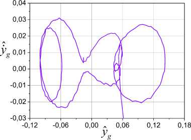
Fig.2. System phase portrait in space R
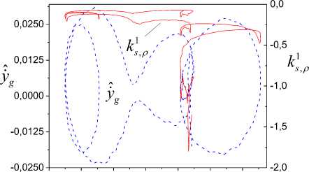
LE identification results are shown in Fig. 3-6. Change of frameworks SKE,, and S 1 is presented in Fig. 3
s,p ks, p where Ak‘ has the form (16), ks is described by expres sion (13), and ks1( t, p) =
p ( y g ( t ) ) t
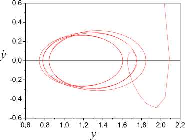
Fig.1. Phase portrait of system
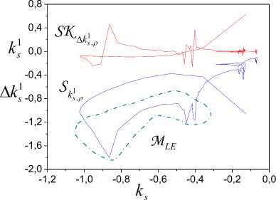
Fig.3. LE set
Apply the model (7) to obtaining of the general solution from y(t) on the time gap [5; 40] s. The model (7) has the form yq (t) = AT [1 u(t) u(t)]T, Aq = [0,302; 0,189; -0,203]T .
The coefficient of determination is 0.95. The estima-
We determine by Lyapunov exponents set
Mle ={-1.8, [-1.21, -0.88]} on the basis of the analysis SKEk, . Apply the theorem 1 and obtain that the system order is 2. The upper estimation for the smallest LE is к =-1.8. The mobility admissible limit of the higher indicator x is -0.8 . We have another LE set on the interval ks g [-0.2, -0.13] that confirms the inference in the remark 3.
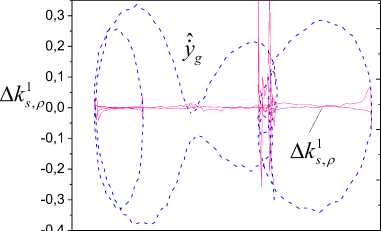
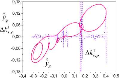
X -adequacy estimation results of the LE set are presented in Fig.4, 5. X -adequacy estimations in spaces R and R л = ( y, g , A k ‘ , p ) on the time gap [3, 55] s are shown in Fig. 4. The function f regions Di coincide with an -almost periodicity regions of the framework 5 1 k s , p that x -adequacy of LE estimations confirms.
0,0250
0,0125 y g
0,0000
-0,0125
, -0,0250
-0,12 -0,08 -0,04 0,00 0,04 0,08 0,12
/X yg
Fig.4. X -adequacy estimation results in spaces Ry and RA
-0,12 -0,08 -0,04 0,00 0,04 0,08 0,12
y g
Fig.5. X -adequacy estimation results in spaces Ry and R 1
Fig. 5 represents x -adequacy results of Lyapunov exponents estimations in spaces Ry and R ,1 = ( y ,, k 1 J .
y k g s , P
They are correlated with results presented in Fig. 4. Frameworks reflect the state of LE identification system for t > 3 s.
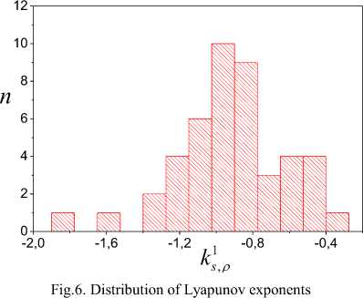
LE distribution example on the basis of parameter (22) change analysis is showed in Fig. 6.
The histogram method [20] confirms obtained estimations x . The histogram gives to a spectrum of Lyapunov exponents. The LE distribution example on the basis of parameter (22) change analysis is showed in Fig. 6, where n is the number of hits x in the specified interval.
We will return to the original system (1). The second order system (1) has the following parameters
A( t ) =
0 1
_ a 1( t ) a 2 ( t ) J ,
ax ( t ) = - 3 + 0.2 sin(0.02 nt ) , аг (t ) = - 4 + 0.3 sin(0.04 nt ) .
Matrix A eigenvalues changed in the range:
\ ( t ) e [ - 1.325, - 0.819 ] , ^ ( t ) g [ - 2.37, - 3.48 ] .
Modeling results show that the proposed approach allows obtaining LE estimations.
Apply the approach stated in the first part of this section to LE identification. Find the model (7) for obtaining of the general solution for y, y. Apply operation of numerical differentiation to calculation y . Models (7) have form yq (t) = [0.75; 0.07; -0.22] [1 u(t) U(t)f ,
\ (t) = -1 + 0.2sin(0.02^t), yq (t) = [-0.394; -0.059; 0,078][1 u (t) U (t )]r.
The determination coefficients for these models are 0.99. Next, find estimations for system free motion.
Consider frameworks SK^k, , S 1 , presented in Fig. 8, s,P ks, p and apply them to system order estimation. The analysis of change SK 1 will show that the system has the third A ks, p order. We obtain Lyapunov exponent set
^ ( t ) = - 2 + 0.3sin(0.04 ^ t ),
^ ( t ) = - 3 + 0.2sin(0.06 ^ t ).
MLE = {-2.04; -1.842; -1.77; -1.167; -0.878} on the basis of the analysis SK 1 and SK 2 . The up-
A ks, p ^ks, p per bound for the smallest LE is к = -2.04. The mobili ty admissible limit of the higher indicator % is —0.8.
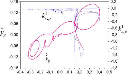
Fig.9. % -adequacy estimation results in spaces Ry and R ^1
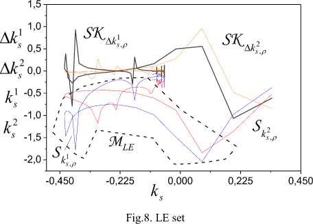
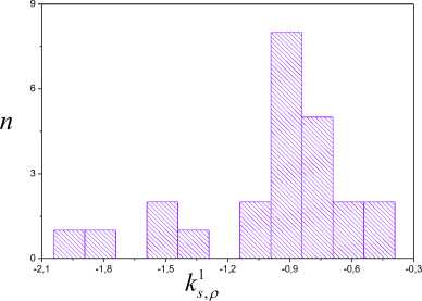
Fig.10. Lyapunov exponent distribution
% -adequacy check results of Lyapunov exponents are presented in Fig. 9, 10. We see that estimations are % -adequate. Fig.10 represents Lyapunov exponent distribution. It coincides with the set M . The framework S
LE yˆ,y form (Fig. 8, 9) is defined by system (1) parameters.
yˆg
Fig.8. % -adequacy estimation results in spaces Ry and RA
The initial system has following eigenvalues of the state matrix
So, modeling results show that the proposed approach allows obtaining estimations Lyapunov exponent estimations. It gives a complex assessment of the Lyapunov exponent spectrum. This is the main advantage of this method. The basis of this method is frameworks describing to the LE dynamics change. The application of proposed frameworks gives to criteria for LE set selection. We show that the obtained LE set has % -adequacy property. The histogram method confirms obtained results. Proposed mathematical procedures give numerical confirmation of LE characteristics obtained theoretically by [19]. The structural approach gives the lineal distribution of a dynamic system.
-
XI. C onclusion
Lyapunov exponents (LE) identification problem of dynamic systems with periodic coefficients is considered under uncertainty. The approach to LE identification applied in nonlinear dynamics problems is proposed. It differs from the great number of existing approaches based on the analysis of a time series and Takens theorem. The problem solution is based on the formation of the set containing information on system general solution. We construct the phase portrait which analysis allows making the conclusion about system properties. The concept απ -almost periodic function in Bohr's sense is introduced as considered processes are not periodic in the standard sense. We propose frameworks reflecting dynamics of Lyapunov exponent change. Upper bound for the smallest LE and mobility limit for the large LE are obtained and the indicator set of the system is determined. The graphics criteria based on the analysis of framework special class properties are proposed for the adequacy estimation of obtained indicators. The histogram method is applied to check of the obtained estimation set. We show that the dynamic system can have Lyapunov exponent set.
References About Lyapunov exponents identification for systems with periodic coefficients
- K. Thamilmaran, D.V. Senthilkumar, A. Venkatesan, M. Lakshmanan, “Experimental realization of strange non-chaotic attractors in a quasiperiodically forced electronic circuit,” Physical Review E, vol. 74, no. 9, pp. 036205, 2006.
- R. Porcher, G., “Thomas Estimating Lyapunov exponents in biomedical time series,” Physical Review E, vol. 64, no. 1, pp. 010902(R), 2001.
- A. Goshvarpour, A. Goshvarpour, “Chaotic Behavior of Heart Rate Signals during Chi and Kundalini Meditation.” International Journal of Image, Graphics and Signal Pro-cessing, vol. 4, no. 2, pp. 23-29, 2012.
- A. Goshvarpour, A. Abbasi and A. Goshvarpour, “Non-linear Evaluation of Electroencephalogram Signals in Dif-ferent Sleep Stages in Apnea Episodes,” International journal of intelligent systems and applications, vol. 5, no. 10, pp. 68-73, 2013.
- J.A. Hołyst, K. Urbanowicz, “Chaos control in economical model by time-delayed feedback method,” Physica A: Statistical Mechanics and its Applications, vol. 287, no. 3–4, pp. 587–598, 2000.
- W.M. Macek, S. Redaelli, “Estimation of the entropy of the solar wind flow,” Physical Review E, vol. 62, no. 5, pp. 6496–6504, 2000.
- Ch. Skokos, “The Lyapunov Characteristic Exponents and Their Computation,” Lect. Notes Phys, vol. 790, pp. 63–135, 2010.
- R. Gencay, W.D. Dechert, “An algorithm for the n Lya-punov exponents of an n-dimensional unknown dynamical system,” Physica D, vol. 59, pp. 142-157, 1992.
- F. Takens, “Detecting strange attractors in turbulence,” Dynamical Systems and Turbulence. Lecture Notes in Mathematics /Eds D. A. Rand, L.-S. Young. Berlin: Springer-Verlag, vol. 898. pp. 366–381, 1980.
- A. Wolf, J.B. Swift, H.L. Swinney, J.A. Vastano, “Deter-mining Lyapunov exponents from a time series,” Physica 16D, no. 16, pp. 285–301, 1985.
- V.A. Bazhenov, O.S. Pogorelova, T.G. Postnikova, “Lya-punov exponents estimation for strongly nonlinear non-smooth discontinuous vibroimpact system,” Strength of Materials and Theory of Structures, 2017, is. 99, pp. 90 – 105.
- A.V. Bespalov, N.D. Polyakhov, “Comparative analysis of methods for estimating the first Lyapunov exponent,” Modern problems of science and education, no 6, 2016.
- V.A. Golovko, "Neural network methods of chaotic pro-cesses processing," In Scientific session of MEPhI-2005. VII All-Russian scientific and technical Neuroinformation scientist(Neuroinformatics)-2005 conference "Neuroin-formatics 2005": Lectures on neuroinformatics. Moscow: MEPhI, pp. 43-88, 2005.
- Y.A. Perederiy, “Method for calculation of lyapunov ex-ponents spectrum from data series,” Izvestiya VUZ. Applied nonlinear dynamics, is. 20, no. 1, pp. 99-104, 2012.
- G. Benettin, L. Galgani, A. Giorgilli, J.-M. Strelcyn, “Lyapunov characteristic exponents for smooth dynamical systems and for Hamiltonian systems: A method for com-puting all of them,” Pt. I: Theory. Pt. II: Numerical appli-cations, Meccanica, vol. 15, pp. 9–30, 1980.
- O. Moskalenko, A. A. Koronovskii, A.E, Hramov, “Lya-punov exponent corresponding to enslaved phase dynamics: Estimation from time series,” Physical review E 92, 2015, 012913.
- Cvitanovi´c P., Artuso R., Mainieri R., Tanner G., Vattay G., Chaos: Classical and Quantum, ChaosBook.org ver-sion16.0, 2017.
- V.V. Filatov, “Structural characteristics of geophysical fields anomalies and their use in forecasting,” Geophysics, no. 4(16), pp. 34-41, 2013.
- B.F. Bylov, R.E. Vinograd, D.M. Grobman, V.V. Nemyt-sky, Theory of Lyapunov indexes and its application to stability problems. Moscow: Nauka, 1966.
- N. N. Karabutov, Frameworks in problems of identification: Design and analysis. Moscow: URSS/Lenand. 2018 (in Russian).
- G. Bohr. Almost periodic functions. Moscow: Librocom, 2009.
