About non-parametric identification of T-processes

Introduction. In numerous multidimensional real processes output variables are available to measure not only at different time periods but also after a long time. This leads to the fact that dynamic processes have to be considered as non-inertial with delay. For example, while grinding the products time constant is 5–10 minutes, and control of output variable, for example fineness of grinding, is measured once in two hours. In this case investigated process can be presented as non-inertial with delay. If output variables of the object are somehow stochastically dependent, then we call such processes T -processes. Similar processes require special view on the problem of identification different from existing ones. The main thing is that identification of such processes should be carried out differently from the existing theory of identification. We should pay special attention to the fact that the term “process” is considered below not as processes of probabilistic nature, such as stationary, Gaussian, Markov, martingales, etc. [1]. Below we will focus on T -processes actually occurring or developing over time. In particular technological process, industrial, economic, the process of person’s recovery (disease) and many others.

Identification of multidimensional stochastical processes is a topical issue for many technological industrial processes of discrete-continuous nature [2]. The main feature of these processes is that vector of output variables x = (x1,x2, ...,xn), consisting of n component is such that the components of this vector are stochastically dependant unknown in advance way. We denote vector of input component - u =(u1,u2, ...,um). This formulation of the problem leads to the fact that the mathematical description of the object is represented as some analogue of the implicit functions of the form Fj (u, x) = 0, j = 1, n . The main feature of this task of modeling is that class of dependency F (•) is unknown. Parametric class of vector functions Fj (u, x, a), j = 1, n , where a is a vector of parameters, does not allow to use methods of parametric identification [3; 4] because class of functions accurate to parameters cannot be defined in advance and well known methods of identifications are not suitable in this case [3; 4]. In this way the task of identification can be seen as solving of non-linear equations:

F j ( u , x ) = 0, j = 1, n (1)

relatively component vector x = ( x 1 , x ₂, ..., x n ) at known values of u . In this case it is expediently to use methods of nonparametric statistics [5; 6].

T -processes. Nowadays the role of identification of non-inertial systems with delay is increasing [7; 8]. This is explained by the fact that measurement of some of the most important output variables of dynamic objects is carried out through long periods of time, that exceeds a constant of time of the object [9; 10].

The main feature of identification of multidimensional object is that investigating process is defined with the help of the system of implicit stochastic equations:

F j ( u ( t -t ) , x ( t ) , ^ ( t ) ) = 0, j = 1, n , (2)

where F j ( • ) is unknown, т is delay in different channels of multidimensional system. Further τ is omitted for simplicity.

In general investigated multidimensional system implementing T -processes can be presented in fig. 1.

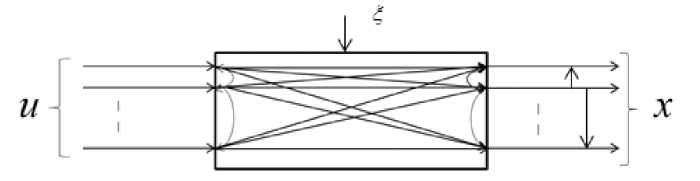
Fig. 1. Multidimensional objects

Рис. 1. Многомерный объект

In fig. 1 the following designations are accepted: u = = ( u ₁, ..., u m ) - m -dimensional vector of input variables,

x = ( x ₁, ..., x n ) - n -dimensional vector of output variables. Through various channels of investigated process dependence of j component of vector u can be presented as dependence on components of vector u: x < j > = f j ( u < ^j > ) ,

j = 1, n .

Every j channel depends on several components of vector u , for example u < ⁵ > = ( u ₁, u 3 , u 6 ) , where u < ⁵ > is a compound vector. When building models of real technological and industrial processes (complexes) often vectors x and u are used as compound vectors. Compound vector is a vector composed from several components of the vector, for example u < j > = ( x 2 , x 5 , x 7 , x ₈ ) or another set of components. In this case, the system of equations will be F j ( u < ^j > , x < ^j > ) = 0, j = 1, n .

T -models. The processes, which have output variables that have unknown stochastic relationships, were called T -processes, and their models were called T -models. Analyzing the above information it is easy to see, that description of the process in fig. 1 can be accepted as a system of implicit functions:

F ( u < ^j > , x < ^j > ) = 0, j = 1n , (3)

where α is a vector of parameters. Then follows the evaluation of parameters according to the elements of training sample u i , x i , i = 1, s and solution of the system of nonlinear interrelated relations (5). Success in building a model will depend on qualitative parametrization of the system (5).

Further we will consider the problem of building T -models under nonparametric uncertainty, when the system (5) is unknown up to the parameters.

Let the input of the object receive the input variables values, which, of course, are measured. Availability of training sample x i , u i , i = 1, s is necessary. In this case evaluation of vector components of output variables x at known values of u , as noted above, leads to the need to solve the system of equations (4). If dependence of output component from vector components of input variables is unknown, then it is natural to use the methods of nonparametric evaluation [5; 11].

At a given value of the vector of input variables u = u ' , it is necessary to solve the system (4) with respect to the vector of output variables x . General scheme of solution of such a system:

1. First a discrepancy is calculated by the formula:

^ j = F j ( ^u < j > , ^x < j > ( i ) , x s , u s ) , ^j = ¹ n , ⁽⁶⁾

where u < j > , x < j > are compound vectors. The main feature of modeling of such a process under nonparametric uncertainty is the fact that functions (3) F j ( u < ^j > , x < ^j > ) = 0, j = 1, n are unknown. Obviously the system of models can be presented as following:

F j ( u < ^j > , x < ^j > , x s ,и s ) = 0, j = U,          (4)

where x_s , u_s are temporary vectors (data received by s time moment), in particular x_s = ( x ₁, ..., x_s ) = = ^{( x} 11 , ^x 12 , ..., ^x 1 s , ..., x 21 , x 22 , ..., x 2 s , ..., ^xn 1 , x n 2 , .", x ns ) , but even in this case F j ( ■ ) , j = 1, n are unknown. In the theory of identification such problems are not solved and are not set. Usually parametric structure is chosen (3), unfortunately it is difficult to fulfill because of lack of apriori information. Long time is required to define parametric structure, that is the model is represented as:

where we take F ( u < ^j > , x < ^j > ( i ) , x_s , й_s ) as nonparametric

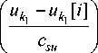
evaluation of regression of Nadaraya–Watson [10]:

j i ) = F j ( ^u < j > , x j ⁽ i ) ) =

= x j

(i) —

s        <  n >

Z x j rnn Ф i = 1          k = 1

' u k - u k [ i ] " _v c ^su k     у

F j ( u < j > , x < j > , a ) = 0, j = 1, n ,           (5)

s < n >

Ф i=1 k=1

' u k - u k [ i ] "

c

V    suk    у

where j = 1, n , , <  m >  is dimension of a compound vec

tor u_k , <  m > <  m , further this designation is also used

for other variables. Bell-shaped functions Ф

' u k - u k [ i ] "

V    suk    7

and parameter of fuzziness c_suk satisfy several conditions of convergence and have the following features:

Ф(■)<”; с;1 J Ф(с;1 (u-u^u = 1;

Q ( u )

^lim s ^„ ^с /Ф( ^c ' ( u ^- u i ) ) = 5 ( u ^- u i ) , Bm s C s = 0, lim s ^„ ^scs = ” .

2. Next step is conditional expected value:

X j = M { x I u < j > , s = 0 } , j = 1, n .           (8)

We take nonparametric evaluation of regression of Nadaraya–Watson as an estimate (8) [10]:

x j =

described, for example, by the following system of equations:

F x1 ^{( X} 1 , x 3 , ^U 1 , u 2 , u 5 ) = ^0;

■ F x 2 ( ^x 1 , x 2 , u 4 , u 5 ) = 0;                      ⁽¹¹⁾

F x 3 ( x 1 , x 2 , x 3 , u 2 , u 3 , u 5 ) = 0-

s          < n >

Х Xj[i] ■П Ф i=1         k =1

< m >

П Ф k 2 =1

s <  n >

ХП Ф

i = 1 k₁ = 1

^uk ^- u ^¹ i n ' ф

^Csu    JA = 1

, j = 1, n , (9)

The system of equations (11) is a dependence, unlike the system (10), known from the available a priori information.

Having got a sample of observation, we can proceed to a studied problem, which is finding the forecast values of output variables x at known input u . First, discrepancies are calculated (7) using the technique described earlier. We introduce discrepancies as a system:

e ₁ ( i ) = F ( x 1 , x 3 , u l , u 2 , u 5 ) ;

where bell-shaped functions Ф ( ■ ) are taken as triangular core:

■ ^E 2 ⁽ i ) = F 2 ( ^X 1 ’ x 2 ’ u 4 ’ u 5 ) ^;

S 3 ( i ) = F ^₃ ( x 1 , x 2 , x 3 , u 2 , u 3 , u 5

1   I uk - "d i ]|   |uk1 - "d i ]|

1, csu             csu

0 I ^uk 1 ^{- u}- d , 1

< 1,

^{1 -}

=1

0,

c su

У.

^Cs S

< 1,

Carrying out this procedure we obtain the value of output variables x under input influences on the object u = u ' , this is the main purpose of a required model, which further can be used in different management systems [8], including organizational one [12].

Computational experiment. For computational experiment a simple object with five input variables u = ( u ₁, u ₂, u 3 , u 4 , u 5 ) taking random values in the interval u e [0, 3] and with three output variables x = ( x ₁, x ₂, x 3 )

where x ₁ e [ - 2; 11], x ₂ e [ - 1; 8], x ₃ g [ - 1; 8] was chosen. We will develop a sample of input and output variables based on a system of equations:

x ₁ - 2 u ₁ + 1.5V ^ T - u 2 - 0.3 x ₃ = 0;

■ x 2 - 1.5 u ₄ - 0.3 ^5 - 0.6 - 0.3 x ₁ = 0;            (10)

x ₃ - 2 u 2 + 0.9д Ц" - 4 u ₅ - 6.6 + 0.5 x ₁ - 0.6 x 2 = 0.

As a result we get a sample of measurements u_s , x_s where u_s , x_s are temporary vectors. It should be noted that the process described by the system (10) is only necessary to obtain training samples, there is no other information about the process under investigation. Dealing with a real object, a training sample is formed as a result of measurements which are carried out with available control measures. In the case of stochastic dependence between output variables, the process is naturally

where s j , j = 1,3 are discrepancies, whose corresponding components of an output vector cannot can’t be derived from the parametric equations.

The forecast for the system (11) is carried out according to the formula (9) for each output component of the object.

First, we present the results of a computational experiment without interference. In this case, values of input variables of the newly generated input variables (not included in the training sample) go to the input of the object. A configurable parameter will be a parameter of fuzziness с_s , which in this case, we take equal 0.4 (the value was determined as a result of numerous experiments to reduce the quadratic error between model and object output [13; 14]) the parameter of fuzziness will be taken the same when calculating in the formulas (7) and (9), sample size is s = 500. Let’s give graphs for object outputs by components x 1 , x 2 and x 3 .

In fig. 2, 3 and 4 the output values of the variables are marked with a “point”, and the output value of the model are marked with a “cross”. The figures demonstrate the comparison of the true values of the test sample of the output vector components and their forecasted values obtained by using the algorithm (6)–(9).

We will conduct the results of another computational experiment, in this case, interference ^ is imposed on values of the vector x components of the object output. The conditions of the experiment: sample size is s = 500, interference acting on the output vector components of an object is ^ = 5 % , parameter of fuzziness is c_s = 0.4 (fig. 5–7).

The conducted computational experiments confirmed the effectiveness of the proposed T -models, which are presented not as generally accepted in the theory of model identification, but as some method of forecasting the output variables of the object at the known input u = u ' . It should be noted that in this case we do not have a model in the sense generally accepted in the theory of identification [15].

Output value

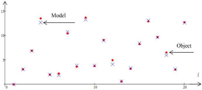
Fig. 2. Forecast of the output variable x 1 with no interference. Error 5 = 0.71

Рис. 2. Прогноз выходной переменной x 1 при отсутствии помех. Ошибка 5 = 0,71

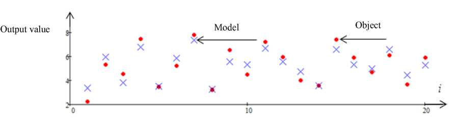
Fig. 3. Forecast of the output variable x ₂ with no interference. Error 5 = 0.71

Рис. 3. Прогноз выходной переменной x ₂ при отсутствии помех. Ошибка 5 = 0,71

Output value

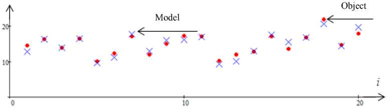
Fig. 4. Forecast of the output variable x ₃ with no interference. Error 5 = 0.71

Рис. 4. Прогноз выходной переменной x ₃ при отсутствии помех. Ошибка 5 = 0,71

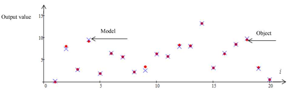
Fig. 5. Forecast of the output variable x 1 with interference 5 %. Error 5 = 0.77

Рис. 5. Прогноз выходной переменной x 1 с помехой 5 %. Ошибка 5 = 0,77

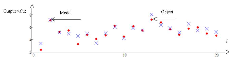
Fig. 6. Forecast of the output variable x 2 with interference 5 %. Error 8 = 0.77

Рис. 6. Прогноз выходной переменной x 2 с помехой 5 %. Ошибка 8 = 0,77

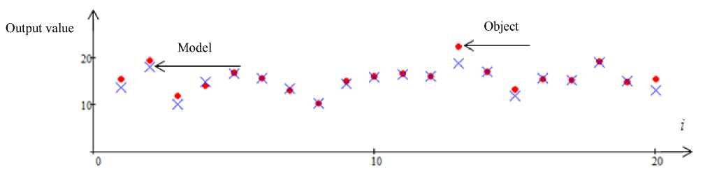
Fig. 7. Forecast of the output variable x 3 with interference 5 %. Error 8 = 0.77

Рис. 7. Прогноз выходной переменной x 3 с помехой 5 %. Ошибка 8 = 0, 77

Conclusion. The problem of identification of non-inertial multidimensional objects with delay in unknown stochastic relations of the output vector components is considered. Here a number of features arise, which mean that the identification problem is considered under conditions of nonparametric uncertainty and, as a consequence, cannot be represented up to a set of parameters. On the basis of available a priori hypotheses the system of equations describing the process with the help of compound vectors x and u is formulated. Nevertheless functions F ( ■ ) remain unknown. The article describes the method of calculating the output variables of the object at the known input, which allows them to be used in computer systems for various purposes. Above some particular results of computational studies are given.

The conducted computational experiments showed a sufficiently high efficiency of T -modeling. At the same time, not only the issues related to the introduction of interference of different levels, different sizes of training samples, but also objects of different dimensions were studied.