About parametric identification algorithms of discrete-continuous processes

Introduction. When researching different processes or phenomena, it is necessary to build models, since we are not always able to conduct experiments with real objects. Herewith various methods of mathematical modelling and identification theory are used. These methods are relevant for studying processes in different branches of human activities (technological, socio-economic processes, etc.). For instance, designing of space vehicles or liquid rocket engines [1; 2].

It is really important to qualitatively determine the mathematical model of the process at the initial stages of the system investigation. These days higher standards of system control are being set. In order to correspond to them, it is necessary to conduct a lot of research and experiments to ensure the construction of an adequate mathematical model of the considering system and to find a more accurate model structure of the object.

Each stage of identification requires different methods due to increasing of the amount of incoming information obtained from the research results. Depending on the amount of information available about the investigated object, the most appropriate method is chosen. Methods for mathematical models determining from the results of experimental researches are the subject of identification theory [3].

Based on the foregoing, it should be added that the construction of a mathematical model depends on the amount of priori information. In this regard, there are two approaches to identification: in a “narrow” and a “broad” sense. For problems in a “narrow” sense there is a vast amount of priori information, whether it is the structure of the system or the class of models to which it refers. This problem statement is close to real conditions and is more applicable in engineering practice [3].

In the “broad” sense of the identification problem there is clear deficit of priori information, or we have access to information only about a qualitative nature object. These methods are time-consuming as they require detailed consideration in each individual case because of the individual features of the objects under study [3].

In conditions of parametric uncertainty parametric identification methods are basically used. Such methods at the first stage assume the determination of the model structure from the available priori information about the object accurate to a parameter vector, which are later estimated with known methods [4]. With parametric modelling, there are cases when priori information is not enough to accurately determine the structure of the model, which can lead to significant errors. In the worst case this can lead to large inaccuracies at the stage of formulating the identification task, which results in an absolutely wrong solution. This problem led to the development of nonparametric identification methods, which have prolifer- ated in recent years [5]. Surely, non-parametric methods allow analysis without using the object model equation. They are more universal and work with greater uncertainty in priori information, this can not be said about parametric methods [6]. However, under conditions of sufficient information parametric methods give better results.

A large number of scientists, both in Russia and abroad, starting from the middle of the twentieth century conducted their studies related to the problem of system identification, since at those particular years it was really significant to broaden knowledge in the field of control [7]. It is commonly believed that Professor Eykhoff P. (Holland) was the first person who systematized the knowledge of the whole variety of identification algorithms and methods. In his monograph [7] he describes the basic concepts of the model, identification problem setting and gives key methods for solving problems for various classes of objects. His book may be useful for those who are working on construction or analysis of processes or phenomena models nowadays. A bit earlier two Professors Andrew P. Sage and James L. Melsa from the USA wrote their book [8], which considers the most well-known methods of identification back then and also conducts their in-depth analysis. Not less important person among foreign scientists who contributed to the development of identification theory is Professor D. Grop (USA). His book [3] complements the knowledge and information which is presented in the book of two Professors Andrew P. Sage and James L. Melsa bringing his new results in the field of identification, and also considering a wider class of different methods that allow us to determine the parameters and structure of the mathematical model.

In Russia the knowledge in the identification sphere was systemized a bit later than abroad, closer to the end of twentieth century. One of the first scientists who wrote a book about constructing mathematical models of complex control objects was Professor N. S. Raibman. In his pamphlet [9], as the author himself called it, N. S. Raib-man describes some of the basic concepts and methods of identification which are intended basically for nonspecialists in the control sphere. Thus, the professor tries to popularize the understanding of the methodology for constructing mathematical models. We would also like to mention proceedings of Professor Sh. E. Shteynberg, who tried to summarize the overwhelming majority of identification methods, possible to be used in engineering practice. His book [10] is aimed at considering the methods which are implemented in industrial enterprises, where there are some missed measurements, noise in the object, the correlation of this noise in time with each other. Therefore, it is applicable to specialists developing control systems. However, the professor’s proceedings can be also useful for an ordinary student. Among other things we should say about the Russian scientist, who made a great contribution to the development of identification and whose work would be wrong not to mention. It is Professor Ya. Z. Tsypkin. His book [4] can be called fundamental as it describes a large range of nuances that appear during the identification algorithms formation. Also, the question of the most optimal identification algorithms selection is considered from various sides. In addition, the “Information Theory of Identification” is a more modern book that was published at the very end of the twentieth century, which emphasizes its relevance to the present days.

Nowadays, there is an active development of the theory of identification in all directions. Thus, in his work [11] L. P. Myshlyaev and coauthors suggest presenting the identification system as a closed-loop dynamic system where the controlled object is the structure of the object model. This approach will help to avoid using adaptive control methods which are effective only for certain classes of objects. A wide application of parametric identification is found in electromechanical systems. For example, in the paper [12], a parametric identification algorithm of an induction motor with a cage rotor is given, where in some cases it is difficult to obtain information about the values of parameters on the basis of catalogued data or to determine them experimentally with the use of special devices. Therefore, the question of constructing a parametric model is quite relevant in this case.

For particularly complex technical and human-technical systems, intelligent control systems are used that combine a large number of different identification methods what is very important in today’s rapidly developing conditions and a huge flow of information. V. B. Trofimov and S. M. Kulakov write about such systems in their work [13]. The authors present the theoretical and applied fundamental basis of intelligent control systems and also offer to familiarize themselves with algorithms that allow solving the actual tasks of various complex systems monitoring and control. Similar studies have already been conducted earlier in the field of parametric identification. The results are presented in [14].

The Problem Statement. The main goal of the paper is to obtain a parametric estimate of the investigated discrete-continuous process. The case when an error was made at the stage of choosing the model structure was studied. In addition, a nonparametric estimation of the investigated process was constructed. The obtained results are compared with the parametric identification method. The generally accepted flowchart of the investigated discrete-continuous process is shown in fig. 1, where the following notation is used: А is an unknown object functional; y ( t ) e Q( y) c R ¹ is an output process variable; u ( t ) = = ( u i ( t ), i = 1, . ., m ) e Q( u) c R^m is a vector input stimulus; ζ( t ) is a vector random stimulus; t is a continuous time; H^u , H^y are communication channels; h^u ( t ), h^y ( t ) are random measurements noise; { u i , y i , i = 1, …, s } is a training sample, where s is a sample size.

Computational experiment. Suppose that the examined object in the computational experiment framework is described by the following equation:

y ( t ) = a 1 ■ u 1 ( t ) + a ₂ ■ [ u 2 ( t )]² +

+ a₃ ■ sin[ u ₃( t )] + a 4 ■ u ₄( t ) + £( t ),            (1)

where (α 1 , α 2 , α 3 , α 4 ) = α – are the coefficients of the studied object; ζ( t ) – is noise with mean value equals zero which was generated in the following way:

^ t ) = y ( t ) ■ c ( t ) ■ k ,                     (2)

where c ( t ) – is a normal distributed random variable in the interval of [–1;1]; k – is the noise level.

Let us assume the model equation has the following form:

y 1 ( t ) = а ₃ ■ U 1 ( t ) + (X₂ ■ [ u 2 ( t )]² +

+ a ₃ ■ sin[ u ₃ ( t )] + a ₄ ■ u ₄ ( t ).                (3)

Next, we suppose such situation when in the modelling process an error was made in the structure with u ₂ and then the following equation now describes the model:

y₂ ( t ) = (X 1 ■ u 1 ( t ) + (i₂ ■ [ u ₂ ( t )]³ +

+ ₃ ■ sin[ u ₃ ( t )] + a ₄ ■ u ₄ ( t ).                (4)

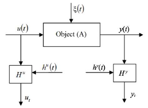
Fig. 1. Flowchart of investigated process

Рис. 1. Схема исследуемого процесса

The next step is to estimate the parameters a 1 , a ₂ , a ₃ and a ₄ based on the available sample {y i , u 1 i , u 2 i , u 3 i , u 4 i , i = 1, …, s }. There is a large number of methods for obtaining parameter estimates, for example, the leastsquares criterion (hereinafter LS criterion). We will use this criterion. The least-squares criterion is presented below:

1 ^s

F (a) = - ^ ( y i - y . )²----->min, (5)

^s i = 1                         ^a

where yi - are model output values; a = ( a 1 , a ₂, a₃,

a₄ ) - are unknown coefficients.

Let us assume the relative approximation error, according to which the deviation of the output values of the models from the output values of the object will be calculated, in the following form:

W =

s

¹ 1 ( у,- y i )²

s i = 1

s

\ т E⁽ m . - y . ) i s -¹ i = 1

^, 2

where m ˆ _y – is the expectation estimation of the object

output.

The form of the nonparametric model constructed for the examined process is presented below [15]:

У ( U ) =

s 4

E у.Пф

i = 1     j = 1

u j

^^^^^^B

c

uji

s 4

E№ i = 1 j = 1

u j

where c s – a blur parameter and Ф(•) – a kernel function satisfy convergence conditions [15].

Kernel Ф(•) has the parabolic form:

Ф ( Z ) = ^

(0.75 - ( 1 -I z\ ) 2

0,

I z l ⁵ 1,

I z >  1,

,          u - u, where z = -

cs

The computational experiment demonstrates the influence of the error, which was made at the stage of selecting the model parametric structure on the final ^odeling results. As the first experiment, we generate the output of the object (1), in which the input variables u j , j = 1, …, 4, are set by uniform-distributed law pseudorandom numbers in the interval of [0,3]. The coefficients of the investigated object will be taken as: α₁ = 7, α₂ = 3, α₃ = 10, α₄ = 11. Using LS criterion (5) for (3) and (4) we get the values of the object estimated coefficients. Substituting these values in (3) and (4) we obtain the values of the model outputs.

In fig. 2 the results are represented, where each timestep corresponds to the values of the object and model outputs obtained from the condition that the sample size is s = 100, and the noise level is 5 %.

The relative approximation error for the model (3) calculated using (6) equals: W 1 = 0.09, but for model (4) equals: W ₂ = 0.14.

Despite the fact that there is an error in the model structure (4), the results which are shown in fig. 2, as well as the value of the error W 2 , indicate that the model describes this object well. This can be explained by presenting the values of the coefficient estimates. For the model (3): <х 1 = 6.95, 2 = 3.038 , <1 3 = 9.986, 4 = 11.013 , for the model (4): 61 1 = 7.37 , a ₂ = 1.06, 3 = 11.37 , a ₄ = 11.19 . As it is evident, the coefficients values at the parameter u 2 differ the most. We construct a graph that visualizes the dependence of the outputs (1), (3) and (4) on the input variable u 2 . For the examined equations we assume u 1 ( t ) = u 3 ( t ) = u 4 ( t ) = 1.5; u 2 will generate using uniform distribution by pseudorandom numbers in the interval of [0;3]. In fig. 3 the results of this experiment are shown.

All above conclusions indicate a feature of the LS criterion which is as follows: even if the model structure is chosen incorrectly at first, the criterion will try to correct it by decreasing or increasing one or another coefficient to make the final model output correspond to the object output in the best way.

The error value (6) can change due to a different sample size. In fig. 4 we consider the dependence of these parameters on each other for models of the form (3) and (4) at a 5 % noise level.

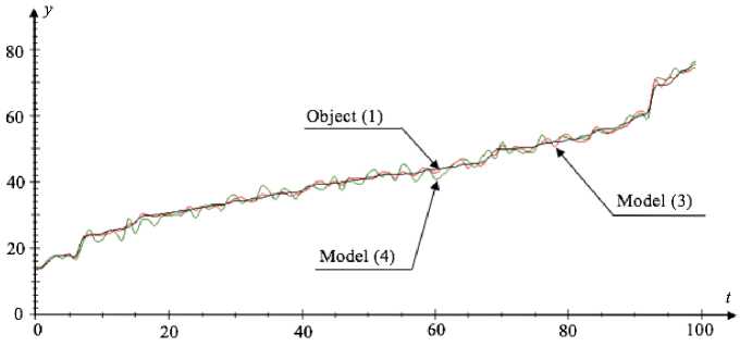
Fig. 2. Graphical dependence of the object (1) and the models (3), (4) outputs in each time-step

Рис. 2. График зависимости выходов объекта (1) и моделей (3), (4) в каждый такт времени

The above given results (fig. 4) show that with the sample size increase, the modelling error tends to one average value.

Among other things, the error (6) changes when the noise level is changed. We investigate this dependence for a sample size s = 100 and summarize the results in tab. 1.

According to the results given in tab. 1, we can assume that for the model (3) and model (4) the error increases with the noise level increase, but for the second case it is more.

As the second experiment, we generate an object with input variables u j , j = 1, …, 4 which are set using uniform distribution by pseudorandom numbers in the interval of [–3;3]. Similar to the first experiment, we graph the object output (1) dependence on the models outputs (3) and (4) at a 5 % noise level and the sample size s = 100, which is shown in fig. 5.

Relative approximation error (6), for the model (3) equals: W 1 = 0.03 and for the model (4) equals: W 2 = 0.42.

The values of the coefficient estimates for the second experiment are as follows. Model (3): a 1 = 7.012, a₂ = 2.99, a₃ = 10.029, a ₄ = 10.984 ; model (4): a 1 = 6.45, a₂ = 0.12, a ₃ = 9.84, a ₄ = 9.82 .

In this case, the interval of input variables generation had a more significant effect on the final output results of the model (4), which is evident in the error value W 2 and fig. 5.

Similar to the above experiment in fig. 6, the graph that shows the dependence of the outputs (1), (3) and (4) on the input of the variable u 2 is given. For the examined equations we assume u ₁( t ) = u ₃( t ) = u ₄( t ) = 1.5, however, now u 2 will be generated by pseudorandom numbers in the interval of [–3;3].

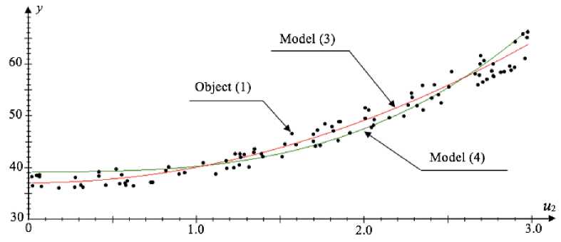
Fig. 3. Dependence of the models (3), (4) and object (1) on u 2 outputs

Рис. 3. Зависимость значений выходов моделей (3), (4) и объекта (1) от u2

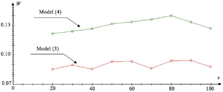
Fig. 4. Relative approximation error graph for different sample sizes

Рис. 4. График относительной ошибки восстановления при различных значениях объема выборки

Dependence of the relative approximation error on different noise levels

Table 1

	W 1 error of the model with correct structure (3)	W 2 error of the model with incorrect structure (4)
Noise level 3 %	0.0611	0.1057
Noise level 5 %	0.0851	0.1356
Noise level 10 %	0.1583	0.1883

The results which are shown in fig. 6, once again indicate that the estimation value of the model (4) coefficient α ˆ ₂ calculated with the criterion (5), is practically equal to zero. Besides that, on the basis of fig. 6 it can be seen that the most qualitative description of the object (1) by the model (4) is only in the interval [–1;1]. Going beyond the limits of this interval, the residual error increases.

Similar to the first experiment, we consider the influence of the sample size on the error value (6) at a 5 % noise level, which is shown in fig. 7.

The results in fig. 7 are similar to the results of the first experiment. The only difference is that for the model (4) the error value (6) has increased.

Now we consider the error value (6) for the different noise levels using sample size s = 100. The obtained results are summarized in tab. 2.

It can be seen from the results presented in tab. 2, the changed interval of generating input object variables affected the error values. For the model (3) a growth in the level noise from 3 % to 5 % as well as from 5 % to 10 % almost twice increases the error value. For the model (4) the error value also increases with noise level increasing, however, because of its large values, this becomes not essential.

As the third experiment, we implement nonparametric modelling of the object (1). The values of the input variables u j , j = 1, …, 4, as in the previous experiments, we will generate pseudorandom numbers using uniform distribution in the intervals of [0;3] and [–3;3].

In the first case (interval [0,3]), we make nonparametric estimate (7) for which the value of the optimal blur parameter c s = 1.1 was calculated. For the second case interval [–3;3] c s = 2.4. Below, fig. 8 and fig. 9 show the results of nonparametric modelling on the assumption that the sample size is s = 100, the noise level is 5 %.

In addition, the error value (6) for different noise levels was calculated. For convenience, we summarize the results in the tab. 3.

Based on the results which are given in tab. 3, we can conclude that the error value (6) for parametric model (4) where the input variables are generated in the interval of [–3,3] is higher than for the model (7). In other cases, the error value (6) for the nonparametric model is higher.

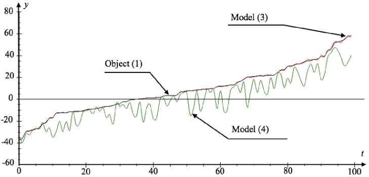
Fig. 5. Graphical dependence of the object (1) and the models (3), (4) outputs in each time-step

Рис. 5. График зависимости выходов (1), (3) и (4) в каждый такт времени

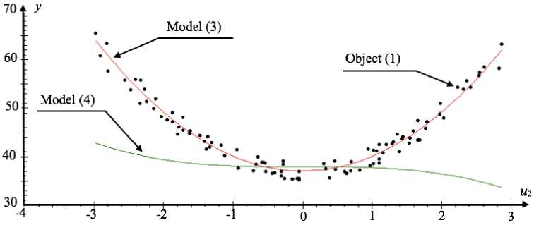
Fig. 6. Dependence of the models (3), (4) and object (1) outputs values on values u 2

Рис. 6. Зависимость значений выходов (1), (3) и (4) от значений u ₂

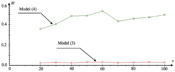
Fig. 7. Relative approximation error graph for different sample sizes

Рис. 7. График относительной ошибки восстановления при различных значениях объема выборки

Dependence of the relative approximation error on different noise levels

Table 2

	W 1 error of the model with correct structure (3)	W 1 error of the model with incorrect structure (4)
Noise level 3 %	0.0151	0.4086
Noise level 5 %	0.0265	0.415
Noise level 10 %	0.0587	0.4651

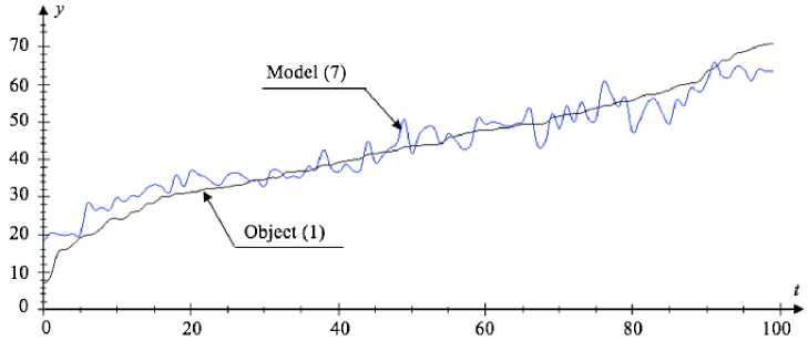
Fig. 8. Graphical dependence of the object output (1) and the model output (7) in each time-step for the interval of generating the input variables [0;3]

Рис. 8. График зависимости выхода объекта (1) и выхода модели (7) от времени для интервала генерирования входных переменных [0;3]

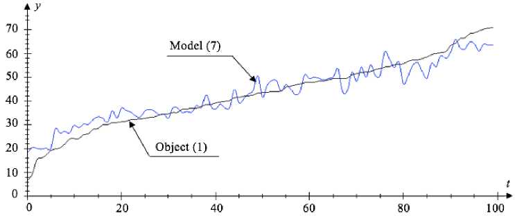
Fig. 9. Graphical dependence of the object output (1) and the model output (7) in each time-step for the interval of generating the input variables [–3;3]

Рис. 9. График зависимости выхода объекта (1) и выхода модели (7) от времени для интервала генерирования входных переменных [–3;3]

Dependence of the relative approximation error on different noise levels for the nonparametric model

Table 3

	The error value (6) of the nonparametric model for the generation interval of input variables [0;3]	The error value (6) of the nonparametric model for the generation interval of input variables [–3;3]
Noise level 3 %	0.268	0.279
Noise level 5 %	0.283	0.314
Noise level 10 %	0.328	0.359

Conclusion. Based on the results of the research, it can be concluded that the minor error made in the process of the model structure definition for one variable does not greatly affect the final results of the model output, since the least-squares criterion neutralizes the error by selecting the required coefficients.

The second experiment results showed us that under certain modelling conditions (for example, the modelling range of input variables values), a model with an error in the structure will describe the object inadequately.

The increase in the sample size affects the error value to a less extent, and with a further increase in the number of observations, this value tends to a specific, average value. The noise levels considered in this work have some effect on the error value.

The third experiment results showed us that the nonparametric model estimates the investigated object accurately enough, but it cannot compete with the correct structure parametric model. Despite this, it is more appropriate to use the nonparametric model in conditions of priori information lack. This fact is confirmed by this experiment, the results of which showed that the value of the modelling error for a parametric model with incorrect structure is higher than for a nonparametric model.