About torsion of parallelepiped around three axis

Introduction. Some tasks of the deformable solid body mechanics are studied rather well. These are so-called statically definable tasks. These tasks deal with torsion of prismatic bars and with plane strain state. They belong to the wide range of tasks – limit state of deformable bodies. The theory of the limit state is one of the fundamental sections of the deformable solid body mechanics [1]. The theory of the limit state deals with statically definable state of solid bodies. In this case the system is closed at the expense of limit conditions and such properties of matter as viscosity, elasticity, etc. cannot influence the limit state. In other words once the limit state has been achieved, the nature of relation between stress and strain does not influence the limit state. Some of such systems are considered in [1–3].

In the first part one system of plasticity equations which describes the limit state is considered. This system can be used for the description of plastic current around three orthogonal axes.

Problem setting. Suppose x = x1, y = x2, z = x3 – orthogonal axes, u, v, w – components of velocity deformation vector, eij – components of velocity deformation tensor, σij – components of stress tensor. Components of stress tensor conforms with the equilibrium equations do ij= о. (1)

On the repeating indexes summing is supposed. Deviator of stress tensor and deformation velocity tensor are coaxial

V iJ -S ij P = ^ e ij ,                     ⁽²⁾

where δ _i j – Kronecker delta; λ – unspecified nonnegative function, 3 p = σ _i j .

Equation system (1)–(2) closes by Mises yield condition

( ° 11 - p ) ² - 1 °” - p ) ² + ( ^o 33 - p ) 2 +

+ 2 (°12 + °13 + °23 ) = 2kS .

It is known [1] that in case of prismatic bar torsion around oz axis, the field of deformation velocities is as folows u = –yz, v = xz, w = w(x,y).(4)

Generalizing ratios (1) we will demand u = u(y,z), v = v(x,z), w = w(x,y).(5)

We will construct the system of equations corresponding to the field of deformation velocities. As a result we receive the following system which will be researched in the study presented

5yt1 +5zt2 =dxp, 5xt1 +5zt3 =dyp, d x T2 + d y T3 = d zp , (T1 )2 + (T2 )2 + (T3 )2 = ks-

The system of equations (6) can be used, in particular, for the description of rectangular parallelogram in the plastic state torsion around three axes (see a figure.).

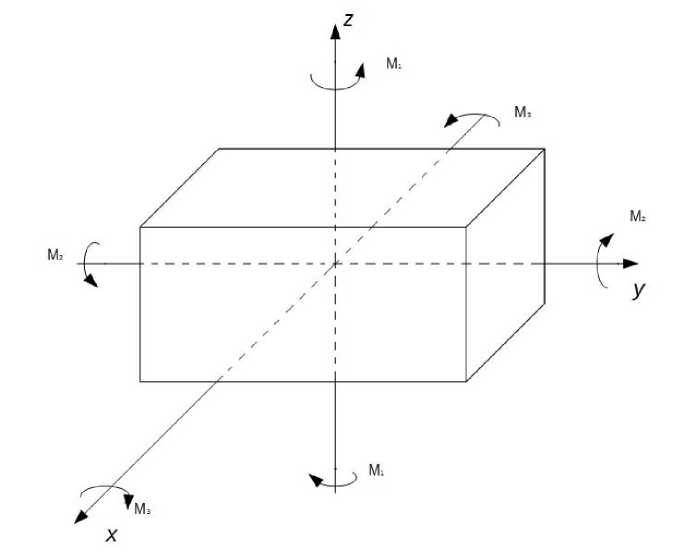
The torsion of parallelepiped around the three axes

Кручение параллелепипеда вокруг трех осей

We will assume that the parallelogram twists around axes of o x , o y , o z in equal and opposite pairs of forces with the moments M 1 , M 2 , M 3 . At the same time there are some limit moments M 1 , M 2 , M 3 when the parallelepiped passes into the plastic state and begins to twist. From the system (6) it is visible that such task is statically definable and can serve for limit moment values finding via formulas

M * = Л ( У т 2 - z т ¹ ) dydz ,

M * = H ( z т¹ — x т 3 ) dxdz ,              (7)

M 3 = If ( x т 3 — У т 2 ) dydz .

Except the moments (7) the body is affected by hydrostatic pressure

Pl ^ = P 0 ,

∑ – lateral surface of a parallelepiped.

We will now study some properties of the system (7).

1. Characteristic surfaces of system (6).

The system (6) contains the finite ratio, connecting values т1, т2, т3. After having differentiated it on x, y, z we receive the system d y т1 + д z т2 = д xP, д x т1 + д z т3 = д yP, д x т2 + д y т3 = д zP, т15хт1 + т*5,т2 + т3д,,т3 = 0,               (8)

xxx т13 y т1 + т2д y т2 + т35 y т3 = 0, т1д z т1 + т2д z т2 + т3д z т3 = 0.

Let’s represent the equation of the characteristic surface of the equation system (9) as

V = v ( x , y , z ) ,                      (9)

Characteristic surfaces of the system (8) are found from the determinant a x V d y V d y V d x V d z V   0

0       т ¹

a z v	0
0	a z v
a x V	a y V	= 0.	(10)
т 2	т 3

Note . It is easy to see that all three latter equations of the system (8) give identical lines in the determinant (10).

Expending the determinant (10) on the last line we receive т1аzV ((dzv)2 - (axv)2 - (dyv)2 ) +

^{+ т} 2 ^а y v ( ( ^a y v ) 2 ^- ( ^a x v ) 2 ^- ( ^a z v ) 2 ) +

^{+ т} 3 ^а x v ( ( ^a x v ) 2 ^- ( ^a y v ) 2 ^- ( ^a z v ) ² ) = 0.

This equation can be written as т1 n3 (2n2 - 1) + т2n2 (2n2 - 1) + т3п (2n2 -1) = 0, (11)

,          d v          d yV          dzV where n1 = .       , n 2 = -=^^=, n 3 = .       .

V ( Vv ) ²        V(vv ) ²        V(vv ) ²

One of solutions of the equation (11) which does not depend on values т ¹ , т ² , т ³ is

2 n i = 1,     i = 1, 2, 3.

Therefore, an angle between the normal to a character-ristic surface v ( x , y , z ) = 0 and vector n equals ±^ 4. Set of elements of the characteristic surface forms the solution cone ± ^ around the direction which is defined by the third root of the equation (11) and depends on tension.

Point symmetries of the equation system (6). Point symmetries are widely used in the studies of differential equations. Necessary data on symmetries and their application to the equations of plasticity and elastic plasticity can be found in [4–8]. Since the system (6) contains finite ratio, we should work with its consequences, which looks like (9), where for convenience the following designations are entered axт1 = qL axт2 = q12, axт3 = q3, axP = q4 etc., q 2+ q 2 = q4, q1+ q 3 = q4, q2+q 2 = q 4, т q1 + т q1 + т q1 = 0, т1 q 2 + т2 q 2 + т3 q 2 = 0,                (12)

т ¹ q 3 +т ² q 2 +т ³ q 3 = 0, 1²2²3²2

( ^т ) ⁺ ( ^т ) ⁺ ( ^т ) = k s .

We will search for point symmetries relative to which the diversity determined by the system of equations (12) is invariant.

According to Lie-Ovsyannikov’s technique, we will search for the admissible operator of point symmetry in view of

X = ^ j ^ + n i -d- , j = 1, 2, 3; i = 1, 2, 3, 4. (13) a x j      ат ⁱ

We continue the operator (13) on the first derivatives by formulas

X = X + g k —,             (14)

d qk where ?k = Dk (ni)-qD (C₽), Dk =^- + qk   .

^{v 7 v 7}         dx_k      дт

With the operator (14) we affect the system of equations (13) and transfer to the diversity set by this system. As a result we receive polynoms of the second level in relation to “internal” – endogenous variables qk2,qk3. “External” – exogenetic variables q1k, qk4 are determined from the system (12) via endogenous variables. In the received polynoms of the second level we equate coefficients to zero in case of the first and second levels of endogenous variables. It allows to receive the redefined system of linear differential equations with respect to coefficients qk2, qk3. Solving this system, obtained is the following result.

Theorem . The system of equations (6) allows Lie algebra L 8 , generated by operators

X. =— i д x i ’	X 4 = x i	д д xi ’	X 5	=_д_ д р ,
X =x — X 12 = x 2 ~ д x 1	д - x-- д x 2	+ т 2	д дт 1	-т 1 —, дт 2 ’
X A X 13 = x 1 - д x 3	д - x 3 — д x 1	+ т1	д дт 3	-т дт 1
X -x A X 23 = x 3 д x 2	д - x 2 — д x 3	■ + т 3	д дт 2	-т 2 А дт 3

Availability of the operators X i , i = 1, 2, 3, 4 means that the system (6) allows shifts and stretching on axes x , y , z Xj = x i + a i , i = 1, 2, 3, x i = x i exp a 4 , shift for hydrostatical pressure p ' = p + a 5 , as well as rotation around three coordinate axes.

• 2.    Invariant solutions of equation system (6).

  • 2.1.    Let’s create invariant solution relative to subalgebra generated by the operator

X з = —.

д z

This type of solution should be searched in the following view д z т rz = rд rP, r д r т r 0 + rд z т0z + 2т r 0 = 0, rд r т rz +т rz = д zP,                     (20)

222 2

^т r 0 ^+т rz ^+т 0 z = ^kS .

In this case тrz is determined from the linear differential equation r5rтrz + r2d2тrz -тrz + r2d2тrz = 0.

Other functions are determined from the system (21).

• 3.    Conservation laws of equation system (6).

Conservation laws are applied to solutions of elastic – plasticity equations. Necessary determination and examples conservation laws usability can be found in [9–15].

Let’s find conservation laws of equation system (6) in the following view axA (т1, т2, т3, p )+a yB (т1, т2, т3, p)+

+ д z C ( т ¹ , т ² , т ³ , P ) = 0.

The equate is done on the account of equation system (6). From this follow the ratio x12 a -т2а pb+т1а pc = 0, x13в - т3аpa+т1аPc = 0, x12в - т2аpa = 0, x12 c -т1а pa = 0,

X13 C + т1д pB = 0, X13 A -т3д pB = 0, т ‘ = т ‘ (x, У), P = P (x, У).

We add (15) in system (6) and we obtain д y T' = д xP, д x T' = д yP, д x т2 + д y T3 = 0,

( ^т ) ⁺ ( ^T ) ⁺ ( ^T ) = k S .

From (16) easily obtain т1 = f (x + y) + g (x - y), P = f (x + y)-g (x - y),

5 т ¹ + д_гт ² = д_х p . yz x

Now functions т2, т3 are determines from the equation systems дx т2 + д y т3 = 0, (т2 )2 + (т3 )2 = kS-(т1 )2.    (18)

The equation system (18) describes the bar torsion in the conditions when the yield stress (limit of fluctuation) depends on variables x , y . These tasks are considered in [4] and in the literature quoted.

• 2.2.    Let’s construct the invariant decision relative to subalgebra generated by the operator X 12. This operator 3

in cylindrical coordinate system r 0 z looks like X ₁₂ = —.

In this case the system (6) will be written as follows

• ^д 0 ^т r 0 ^{+ д} z ^т rz = r ^д rP , r ^д r ^т r 0 ⁺ r ^д z ^т 0 z ^{+ 2 т} r 0 = ^д 0 P ,

r д r т rz + д0т0z +т rz = д zP, тr0 +т rz +т0z = kS .

Invariant solution in this case is determined from the following system

where X_l2 = -т ² д 1 + т 1 д ₂, X ,₃ = -т ³ д 1 + т 1 д 3 . ¹²            т         т ¹³            т         т

Let’s show that these equations are compatible. Suppose д _рА = д _рВ = д _рС = 0, than - one of the solutions

will be the infinite series

A ( S ) , B ( S ) , C ( S ) ,

where S = ( т 1 ) 2 + ( т ² ) 2 + ( т ³ ) 2 , A ( S ) , B ( S ) , C ( S ) -

random differentiable functions.

Remark . Are there other laws? Not stated, but according to the author other conservation laws do not exist.

• 4.    It is clear, for the system (6) tension state is the most relevant. Supposing it is known. Than to find three components of the velocity vector we have three equations

т ¹ =X e ₁₂, т ² =X e ₁₃, т ³ =X e ₂₃,          (21)

where

^{2 e} 12 = ^д y u ^{+ д} x v , ² e 13 = ^д z u ^{+ д} x w , ² e 23 =д z V + д y W.

Let’s show that the equations (21) can be solved

in terms of deformation velocity tensor components. It is known that except the equations (21) deformation velocity tensor components shall satisfy equations of compatibility as well. Owing to ratios (22) and (5) only six

of them remain.

д 2 y e 12 = 0, д 2 z e 13 = 0, д 2^ 23 = 0, ^д x ( ^д x e 23 ^-д z e 12 ^-д y e 13 ) = 0, ^д y ( ^д y e 13 ^-д z e 12 ^-д x e 23 ) = 0, ^д z ( ^д z e 12 ^-д y e 13 ^-д x e 23 ) = 0.

Theorem . The compatibility equations of deformation speeds are done identically.

In this case from (21) we have

12 22222

( ^т ) ( ^е 12 + ^е 13 + e 23 ) = ^kS^e12 ,

22 22222

(т ) (e12 + e13 + e23 ) = kSe23,

32 22222

( ^T ) ( ^e 12 + ^e 13 + e 23 ) = ^kS e 13 ^.

Equation system (24) is a system of linear homogeneous equations relevant to variables e ₁²₂, e ₁²₃, e ₂²₃. Its determinant is

2               \2м2

12   11

T) kS (t )

( ’ 2 ) 2 T ) 2 - k S ( t ² ) 2

T ) 2        ( T ) 2       : ) 2 - k 2

This determinant equals zero as the amount of all lines is equal to zero. It means that the system (24) has only two independent equations for three components of a deformation speed tensor. For example, value e ₂²₃ can be picked up randomly, thus for the given tension state, defined from the system (6), velocity field is defined with the functional arbitrariness.

• 5.    In this part we will consider three-dimensional equations of elasticity in static. The system of equilibrium equations is described using equations (1), relation between components of stress tensor and deformation tensor is as follows

_ ( ^ 11 ^- v ( ^ 22 ⁺^ 33 ) )

£11 =             „

11 E

_ ( ^ 22 ^- v ( ^ 11 ⁺^ 33 ) )

^£ 22 =

_ ( ° 33 ^- v ( ^CT 22 '^ 11 ) )

^£ 33 =

_c _ °12 ^£12 “ , ,

2 ц

_c _ °13 _c _ °23 ^£ 13 “ , , ^£ 23 “ , ,

2ц 2ц where е? deformation tensor components, E, ц, v elastic constants.

Supposing vector deformation components are as follows w1 = w1 (У,z), w2 = w2 (x,z), w3 = w3 (x,z).     (26)

Inserting (26) into (25) we obtain

^1^1

• d, w +o, w, = 12 , d w, +o, w₃ =--- , y 1 x 2 z 1 x 3

2 ц                2 ц

°23

5_Z w , + d w = . ^{z 2} y ³ 2 ц

In this case equation (1) with regard to (26), (27) is as follows d yyw1 + d zzw1 = 0, d xxw2 + d zzw2 = 0, sxwi +d w3 = 0. xx yy

It is shown that components of deformation vector are harmonic functions. The solutions obtained here can be used for the description of elastic status of the parallelepiped twisted around three orthogonal axes. The moments are defined from formulas (7). As £11 + e22 +e33 = 0, dilatation (volume change) is equal to zero. The solution (27) describes vortex movement characterized by the vector ю

	( -г 1	j	k 1
ю =	дх x	d У	d z
	I w 1	w 2	w 3 J

Herewith movement paths will be vortex lines which are defined from the equation dx dy dz w1w2w3.

Conclusion. In the present work for the first time considered is the system which can be used for the analysis of stress state appearing under torsion of the parallelepiped around three orthogonal axes. At that it can be in either plastic or elastic state.