Active Selection Constraints for Semi-supervised Clustering Algorithms

Published Online December 2020 in MECS DOI: 10.5815/ijitcs.2020.06.03

Clustering is the process that divide data into k clusters that group points with similar properties in the sane cluster and different points in different clusters. Clustering based constraints (also known as semi-supervised clustering) improve performance of clustering using must-links ( ML ) and cannot-links ( CL ) constraints. The constraint ML ( x i , x j ) shows that points x i and x j . must be in the one cluster, while a CL ( x i , x j ) shows that points x i and x j must be in different clusters [1, 2].

Semi-supervised clustering algorithms enhancing the clustering accuracy [3, 4, 5]. However, algorithms choose the constraints passively and provided beforehand and selected randomly. Thus, the constraints will be unnecessary, redundant, and can degrade the accuracy of clustering results [6, 7]. Also, it requires the user knows what the most informative constraints are to provide to the algorithm, and this is not feasible in practice because the user cannot browse thousands (or millions) of constraints to select the best ones. We would like to enhance the clustering accuracy by optimizing the constraints selection.

To explain how pairwise constraints can degrade the clustering performance, figure 1 shows a dataset with 36 points and want to divide all points into two equal clusters. We can get the best solutions in figure 1(a . ) and figure 1(b . ). Figure 1(a . ) shows two must-link constraints between the points ( a , c ) and ( c , b ). Figure 1(b) shows different two must-link constraints between the points ( a , d ) and ( d , e ). Thus, from figure 1(a),(b) we can divide the data points into two equivalent groups. However, if we applied the four must-link constraints (figure. 1(c)), we cannot get divide the data into two equivalent groups. We can apply the same observation with cannot-link constraints. In Figure 1(d), two cannot-link constraints CL ( a , f ) and CL ( c , f ) are given. Figure 1(e) presents CL ( f , d ) and CL ( c , d ). However, if we apply the four cannot-link constraints we cannot get the optimal partition (figure 1(f)). This example introduces the problem of how to select the best set of pairwise constraints, as selecting them improperly can degrade the clustering performance [7].

0 0 0 0 0 0	0 0 0 0 0 0	0 ОО b b a c0 ООО ООО ООО (a)	О О О О О О	ООО ООО О О a Оe    d ООО ООО (b)	о о о О о о	о о о о о о	о о о о о о	о о о о о о	о о о о о о с bо a    cо		о о о о о о
									e     d о о о о (c)	о о о о о о
0	0	ООО	О	ООО	о	о	о	о	о о	о о	о
0	0	О. О О a	О	ООО	о	о	о	О	О О	О о	0
0	0	cО	О	ООО	•c	о	о	О	о О. a	.0cо	0
0	0	О -ер О Оf3	О	° ° < d	f f	о	о	О	d О О	f 0 о	о
0	0		О	о о с		о	о	О			0
0	0	ООО (d)	О	ООО (e)	о	о	о	о	о о (f)	о о	о

Fig.1. Examples of pairwise constraints

Active learning is an important issue applied in many supervised learning algorithms where unlabeled instances are numerous and easy to find but labeled instances are, expensive and difficult to found. For example, it is easy to get large number of unlabeled images or documents, whereas determining their types requires manual effort from experienced human annotators.

In this paper, we explain an algorithm that select active pairwise constraints. We select the active constraints based on Radial-Bases Function, we compute the average minimum distance ( lower bound ) and the average maximum distance ( upper bound ) between each two points to choose the most informative constraints that produce an accurate clustering assignment. The proposed algorithm is integrated with different semi- . supervised clustering algorithms. The empirical results on a set of real datasets explain that our algorithm outperforms in term of clustering performance the other methods.

2.    Related Work

Semi-supervised clustering algorithms use the constraints into the clustering process. Existing algorithms classified as metric-based methods or constraint-based methods. The constraints used directly to partition the dataset [1, 2, 8]. While, in metric-based methods, the clustering algorithm used a particular distortion measure the achievement of constraints in the supervised learning [9, 10]. However, Most existing algorithms select the constraints randomly. Thus, these algorithms decreased the clustering performance due to improperly selected constraints.

Active learning can be applied for selecting pairwise constraints in clustering problems [11]. Basu etal. [12] suggested an active selection algorithm based on farthest first query selection (FFQS). Firstly, the authors search the data to find K neighborhoods belonging to different clusters. Then select randomly a set of non-skeleton points and checks them all points in the neighborhood to find ML constraints. Mallapragada etal. [13] improved FFQS by introducing Min–Max measure. Their method modifies the Consolidate phase by selecting the data point with maximum uncertainty. However, these methods do not work well with high dimensions data or unbalanced clusters.

Vu et al. [14] applied an active method that candidate the good query of the dataset based on k -nearest neighbor graph ( k -NNG) and generate the constraints. However, this mechanism may generate constraints that degrade the clustering performance. Xiong et al. [15, 16] select the informative point to form queries accordingly. However, selecting only one point can become very slow for generating the constraints.

Xiong et al. [17] used an active semi-supervised algorithm based on the principle of uncertainty reduction. Wei et al. [18] proposed a filtering active submodular selection (FASS), that combined the uncertainty sampling method with a submodular framework to select examples with equivalent distribution to the unlabeled examples. Yanchao et al. [19] proposed an active learning method that learning from embeddings of deep neural network to use uncertainty and influence of examples.

Most existing algorithms use the constraints in a passive manner. Therefore, selecting the most “valuable” constraints becomes a crucial issue. Also, it is difficult to check all data instances to select the good constraints. Thus, we propose an algorithm that actively select the constraints as maximally informative and without any conflict instead of chosen at random.

3.    Active Pairwise Constraints

We show how to select pairwise constraints effectively to enhance the clustering accuracy. The main point we aim to explained is how to choose the required constraints that improve the performance. We generate an active pairwise constraints, i.e. active must-link (AML) and active cannot-link (ACL) that should be actively selected instead of randomly selected. If instances xi and xj are in one cluster for every optimal partition, then we generate AML constraint (AML(xi, xj)). The AML constraints is referred to AM(X). Also, we can generate ACL. If instances xi and xj are in different clusters for every optimal partition, then we generate ACL constraint (ACL(xi, xj)). The ACL constraints is referred to AC(X).

Given a data set X ={ x 1 , x 2 , . . . , x n }, let E ( x i , x j ) be an edge between each two instances ( x i , x j ) with weight w ij = w ( x i , x j ) computed by the Radial-Bases Function RBF as a similarity function between two instances x i and x j .

• -|l* t -* j l|²\

^S« = e^xp (   2 _{o 2}  )                                          (1)

From the graph G , we compute the average minimum distance ( lower bound ) and the average maximum distance ( upper bound ) between each two points as shown in equations 2 and 3 respectively.

vn Min

• ^{1    jn} tj     _t#j

  
  

lower bound = ------n--------- m vn Max

• V ^ /"   1 ^j E ^{n ij} _S1 t _#j

upper bound = -----^------

First our algorithm computes lower and upper bound and initializing AM ( X ) and AC ( X ), then checks every pairwise constraint to select the most informative constraints as shown in Algorithm 1. In our algorithm we have four cases:

• 1-    Add the constraint ml ( x i , x j ) to AM if the similarity functions between x i and x j <  lower bound .

• 2-    Add the constraint ml ( x i , x j ) to AM if we have must-link between points x i and x l ( ml ( x i , x l )) and must-link between points x l and x j ( ml ( x l , x j )).

• 3-  Add the constraint cl ( x i , x j ) to AC if the similarity functions between x i and x j >  upper bound .

• 4-  Add the constraint cl ( x i , x j ) to AC if we have active must-link between points x i and x l ( AML ( x i , x l )) and active

cannot-link between points x l and x j ( ACL ( x l , x j )).

Algorithm 1: Active Constraint Selection

Input :

Must-link: M

Cannot-link: C

Output :

Active Must-link: AM

Active Cannot-link: AC

Begin :

• 1-    Compute lower bound and upper bound values.

• 2-    Initialize AM0 and AC = 0

• 3-    For each constraint ml ( x i , x j )£ M

• (a)    If the similarity between x i , x j < lower bound Add ml ( x i , x j ) to AM .

Else

• (b)    If constraints ml ( x i , x l ) )£ M and ml ( x l , x j ) )£ M Add ml ( x i , x j ) to AM

End if

End for

• 4-    For each constraint cl ( x i , X j )£ C

• (a)    If the similarity between x i , x j > upper bound Add cl ( x i , x j ) to AC .

Else

• (b)    If constraints ml ( x i , x i ) )£ AM and cl ( x i , x j ) )£

AC

Add cl ( x i , x j ) to AC

End if

End for End .

The algorithm checks every pair of points in each constraint. First, it checks whether a new active must-link constraint can be implied by AM (Step 3). If succeeded, add the constraint to AM. Otherwise, check whether an active cannot-link constraint can be directly inferred by AM and AC (Step 4). If succeeded, add the constraint to AC.

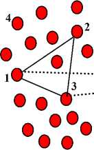
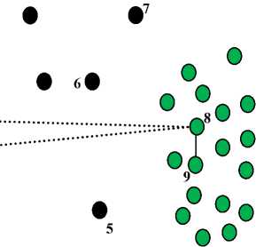
For example, assume we have a dataset with two clusters and has a set of noises as shown in figure 2. From the figure we have 8 ML by solid lines and 5 CL by dashed lines. After applying our algorithm only 4 constraints will be selected as active must-link constraints (( x 1 , x 2 ), ( x 1 , x 3 ), ( x 2 , x 3 ), and ( x 8 , x 9 )) and 2 constraints as active cannot-link constraints (( x 1 , x 8 ) and ( x 3 , x 8 )) as shown in figure 3. The must-link constraint ml ( x 8 , x 9 ) is selected as AML where the similarity functions between x 8 and x 9 smaller than the lower bound value (Step 3(a)). And, the must-link constraints ml (( x 1 , x 2 ), ( x 1 , x 3 ), and ( x 2 , x 3 )) are selected as AML where their instances have must-link constraint with shared point (Step 3(b)). Similarly, the cannot-link constraint cl ( x 1 , x 8 ) is selected as ACL where the similarity functions between x 1 and x 8 greater than the upper bound value (Step 4(a)). And, the cannot-link constraint ( x 3 , x 8 ) is selected as ACL where there is a shared instance ( x 1 ) with AML ( x 1 , x 3 ) and ACL ( x 1 , x 8 ) (Step 4(b)). Figure 3 shows the clustering results using active constraints as we have two clusters and some noises (black circles).

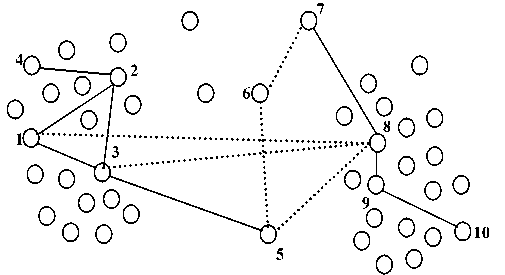
• Fig.2.    Two cluster dataset with set of constraints

  
  
  
  

  о

  • 10

  
  

• Fig.3.    The clustering results of the dataset in figure 2

4.    Experiments

In this section, we present the clustering accuracy and efficiency on a set of data sets from the UCI repository as shown in Table 1.

Table 1. The Data Sets from UCI repository

Dataset	# Instances	#Dimensions	#Clusters
Ecoli	336	8	8
Heart	270	13	2
Protein	116	20	6
Sonar	208	60	2
Breast	569	30	2
Segment	2310	19	7

In all experiments, we use MPCKMeans as a well-known semi-supervised clustering algorithm and compare our proposed algorithm with a number of related state-of-the-art methods as follows:

• •    Random: a baseline in which constraints are randomly selected.

• •    NPU: a neighborhood-based approach that incrementally expands the neighborhoods by selecting a single instance to query each time [15].

• •    FASS: a framework that applies submodular data subset selection [18]

• •    ASCENT: an active learning method based on deep neural network [19]

• 4.1.    Evaluation Metrics

• 4.2.    Evaluation Results for Constraint Selection Methods

To measure the performance of clustering algorithms, we use Normalized Mutual Information (NMI):

1(X;Y)

NMI — (_H(_X)_+H(y))                                                   ⁽⁴⁾

where I ( X ; Y ) = H ( Y ) - H ( Y | X ) is the mutual information between the random variables X and Y, H( Y ) is the Shannon entropy of Y , and H( Y | X ) is the conditional entropy of Y given X .

We explain the results which compare our algorithm with other constraint selection algorithms. We will refer to our algorithm as Active Pairwise Constraints (APC) algorithm.

Figure 4 shows the performance on a different dataset to explain the comparison between the proposed algorithm (APC) and the other algorithms. In the figure, the horizontal axis indicates the set of selected constraints and the vertical axis indicates the clustering performance (NMI) by running MPCKmeans with the selected constraints.

As shown in figure 4, APC consistently performs better than the baselines. In comparison, the NPU method obtains better results with MPCKMeans for the Heart and Protein datasets. For dataset with a small number of clusters (e.g. Heart dataset), the NPU method able to improve the clustering performance. While, in the case of more complex datasets (e.g. Breast, and Segment datasets), the NPU method degrades the performance while including more constraints. In comparison, the FASS and ASCENT methods can improve the clustering performance consistently with increasing the number of pairwise constraints. ASCENT method obtains better results than APC with small number of constraints (e.g. Ecoli, Protein, Sonar, and Segment datasets). However, drop inefficiency with increasing the number of constraints makes the proposed algorithm better than ASCENT. In comparison with FASS method that generally outperforms Random, and NPU methods. FASS is generally able to improve the clustering performance consistently as increasing the number of constraints. However, the proposed algorithm is more effective than other algorithms. For example, the NMI of APC is (0.87, 0.83, 0.68, 0.94, 0.97, and 0.75) after selecting 150 active pairwise constraints for the data set (e.g. Ecoli, Heart, Protein, Sonar, Breast, and Segment) respectively, which wins the best of compared methods over (0.04, 0.09, 0.03, 0.04, 0.04, and 0.02) respectively as shown in figure 4. While, selecting constraints randomly, degrades the performance in some datasets as we include more constraints, as shown in the ecoli and heart datasets. The experimental results demonstrate that selecting active pairwise constraints improve the clustering performance.

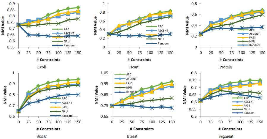
Fig.4. Comparison of normalized mutual information on different datasets

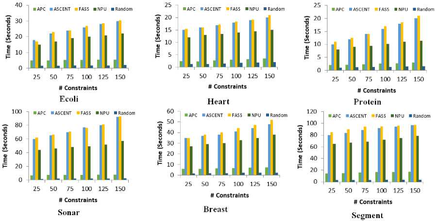
Fig.5. Comparison of average run time over different number of constraints.

One of the primary motivations of the proposed algorithm is to reduce the computation when increasing number of constrains. Figure 5 shows the CPU running time of the proposed algorithm with baseline algorithms on a Intel Core i5 (3.5 GHz) and 8 GB main memory.

From the figure, when adding more constraints, the CPU running time of the proposed algorithm increases slowly. For example, for the Heart dataset, ASCENT, FASS, and NPU takes about (15.2, 16.6, 12.8) milliseconds with 25 constrains respectively, while APC needs only 2.4 milliseconds. While, after applying 150 constraints, ASCENT, FASS, and NPU takes about (20.4, 23.1, 15.6) milliseconds respectively, while APC needs only 3.7 milliseconds. For a complex dataset like Segment, ASCENT, FASS, and NPU takes about (77.4, 83.3, 68.4) milliseconds with 25 constrains respectively, while APC needs only 16.6 milliseconds. While, after applying 150 constraints, ASCENT, FASS, and NPU takes about (98.4, 101.2, 82.4) milliseconds respectively, while APC needs only 17.8 milliseconds. Finally, the required time for our algorithm increases moderately when increasing the number of constrains. While, other methods increase tremendously. Also, we can see that Random methods is the fastest method as it does not require any time to select the constraints.

• 4.3.    Evaluation Results for Clustering Algorithms

For evaluating the proposed algorithm, we compared its performance with well-known unsupervised and semisupervised clustering methods as the base learner. We use (K-means and EM) as unsupervised clustering methods, (MPCKmeans and Constrained EM) with 10% random constraints as semi-supervised clustering methods.

We compute the average performance across 20 independent runs. From Tables 2, the constraint-based clustering algorithms are not always outperforming the corresponding unsupervised clustering algorithms (e.g Ecoli, Sonar and Breast dataset). For example, the average NMI of MPCKmeans and Constrained EM is (0.68 and 0.64) respectively on ecoli dataset. While, Kmeans and EM methods are more effective (0.73 and 0.74) respectively. It is interesting to note that the random selection of constraints degrades the clustering performance. The proposed method achieved the highest NMI results on all the datasets. Among all the results, we can see that clustering with active pairwise constraints outperformed other unsupervised and semi-supervised algorithms on each dataset.

From Table 3, it is clear that constraint-based clustering algorithms need more CPU time than unsupervised algorithms, as the performance of unsupervised clustering algorithms don’t base on selecting pairwise constraints. Also, the results show that our active pairwise constraints selection method is slower than random method that selects set of constraints randomly without performing additional CPU time for selecting constraints. For example, the computation time of MPCKmeans and Constrained EM are (16.34 and 15.12) millisecond respectively on segment dataset. While, MPCKmeans and Constrained EM with APC methods are (17.32 and 16.22) millisecond respectively.

Table 2. The average NMI of different algorithms.

Dataset	Kmeans	MPCKmeans	MPCKmeans with APC	EM	Constrained EM	Constrained EM with APC
Ecoli	0.731±0.015	0.68±0.032	0.764±0.028	0.742±0.056	0.647±0.073	0.758±0.025
Heart	0.334±0.063	0.418±0.041	0.645±0.050	0.445±0.014	0.473±0.013	0.598±0.059
Protein	0.236±0.043	0.386±0.022	0.614±0.078	0.542±0.052	0.492±0.046	0.642±0.012
Sonar	0.632±0.035	0.513±0.081	0.792±0.033	0.724±0.042	0.673±0.081	0.833±0.024
Breast	0.821±0.028	0.742±0.036	0.912±0.024	0.844±0.059	0.779±0.041	0.928±0.046
Segment	0.563±0.034	0.668±0.053	0.744±0.023	0.668±0.046	0.734±0.023	0.808±0.065

Table 3. Average run time (millisecond) of different algorithms.

Dataset	Kmeans	MPCKmeans	MPCKmeans with APC	EM	Constrained EM	Constrained EM with APC
Ecoli	3.46	5.44	6.12	3.72	5.13	5.76
Heart	1.65	3.25	4.26	2.12	3.63	4.65
Protein	1.32	2.57	3.15	1.70	2.18	3.65
Sonar	2.23	7.42	7.87	2.87	7.34	8.03
Breast	2.21	5.78	6.04	3.65	5.13	6.23
Segment	5.43	16.34	17.32	6.23	15.12	16.22

5.    Conclusion and Future Works.

In this paper, we presented the active constraint selection for semi-supervised clustering algorithms. We introduced active pairwise constraints ( AML and ACL ) which would not conflict with each other to improve the clustering performance. The proposed algorithm can be applied on any semi-supervised clustering methods. The experiments conducted on a set of real datasets with MPCKmeans and constrained EM show that the proposed algorithm can select the best informative pairwise constraints and outperforms in term of clustering performance the baseline methods. In future work, we would like to work on the problem of incremental growing constraint set for streaming data. To address this problem, we interest to apply an incremental semi-supervised clustering method.