Adaptive Forecasting of Non-Stationary Nonlinear Time Series Based on the Evolving Weighted Neuro-Neo-Fuzzy-ANARX-Model

Published Online October 2016 in MECS

Mathematical forecasting of data sequences (time series) is nowadays well studied and there is a large number of publications on this topic. There are many methods for solving this task: regression, correlation, spectral analysis, exponential smoothing, etc., and more advanced intellectual systems that require sometimes rather complicated mathematical methods and a high qualification of a user. The problem becomes more complicated when analyzed time series are both non-stationary and nonlinear and contain unknown behavior trends as well as quasiperiodic, stochastic and chaotic components. The best results have been shown by nonlinear forecasting models based on mathematical methods of Computational Intelligence [1-3] such as neuro-fuzzy systems [4-5] due to their approximating and extrapolating properties, learn ing abilities, results ’ transparency and interpretability. The models to be especially noted are the so-called NARX-models [6] which have the form

У ( k ) = f ( y ( k - 1 ) ,..., y ( k - n_y ) , x ( k - 1 ) ,..., x ( k - n x ) )

where y ( k ) is an estimate of forecasted time series at discrete time k = 1,2,... ; f ( • ) stands for a certain nonlinear transformation implemented by a neuro-fuzzy system, x ( k ) is an observed exogenous factor that defines a behavior of y ( k ) . It can be noticed that popular Box–Jenkins AR-, ARX-, ARMAX-models as well as nonlinear NARMA-models can be described by the expression (1). These models have been widely studied; there are many architectures and learning algorithms that implement these models, but it is assumed that models’ orders n and n are given a priori. These orders are previously unknown in a case of structural non-stationarity for analyzed time series, and they also have to be adjusted during a learning procedure. In this case, it makes sense to use evolving connectionist systems [7-10] that adjust not only their synaptic weights and activation-membership functions, but also their architectures. There are many algorithms that implement these learning methods both in a batch mode and in a sequential mode. The problem becomes more complicated if data are fed to the system with a high frequency in the form of a data stream [11]. Here, the most popular evolving systems turn out to be too cumbersome for learning and information processing in an online mode.

As an alternative, a rather simple and effective architecture can be considered. It’s the so-called ANARX-model (Additive NARX) that has the form [12, 13]

y ( k ) = f ( y ( k - 1 ) , x ( k - 1 ) ) + f , ( y ( k - 2 ) , x ( k - 2 ) ) + ...

n

...+ f„ (у (к -n), x(к -n)) = ^ ft (y (к -1), x(к -1)) I=1

(here n = max{n, nx} ), an original task of the forecasting system’s synthesis is decomposed into many local tasks of parametric identification for node models with two input variables y (k -l) , x (k -1) , l = 1, 2,..., n.

....

Authors [12, 13] used elementary Rosenblatt perceptrons with sigmoidal activation functions as such nodes. The ANARX-model provided a high forecasting quality, but generally speaking it requires a large number of nodes in its architecture [14].

Some synthesis problems of forecasting neuro-fuzzy [15] and neo-fuzzy [15-17] systems based on the ANARX-models are considered in this work. These systems avoid the above mentioned drawbacks.

Since we consider a case of stochastic nonlinear dynamic signals in this article, the basic novelty has to do with defining a model’s delay order in an online mode.

The remainder of this paper is organized as follows: Section 2 describes an architecture of a neuro-fuzzy-

ANARX-model. Section 3 describes an architecture of a neo-fuzzy-ANARX-model. Section 4 presents a weighted neuro-neo-fuzzy-ANARX-model. Section 5 presents several real-world applications to be solved with the help of the proposed system. Conclusions are given in the final section.

• II.    A N EURO -F UZZY -ANARX-M ODEL

An architecture of the ANARX-model is shown in Fig.1. It is formed by two lines of time delay elements z ¹ ( z ¹ y ( k ) = y ( k — 1 ) ) and n nodes N ^{[ l ]} which are simultaneously learned. These nodes are tuned independently from each other. By adding new nodes or removing unnecessary ones, it doesn’t have any influence on other neurons, i.e. the evolving process for this system is implemented by changing a number of the nodes.

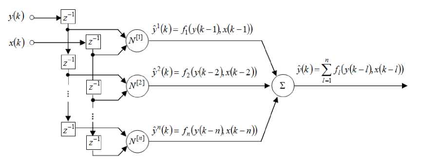
Fig.1. The ANARX-model.

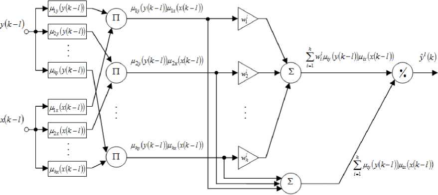
Fig.2. A neuro-fuzzy node of the ANARX-model.

It’s recommended to use a neuron with two inputs (its architecture is shown in Fig.2) as a node of this system instead of the elementary Rosenblatt perceptron. As one can see, this node is the Wang–Mendel neuro-fuzzy system [18] with two inputs. It possesses universal approximation capabilities and is actually the zero-order

Takagi–Sugeno–Kang system [19, 20]. A twodimensional vector of input signals z_t ( k ) = ( y ( k - 1 ) , x ( k - 1 ) ) T is fed to an input of the node N ^{[ 1 ]} , l = 1, 2,..., n,.... The first layer contains 2 h membership functions M iy ( y ( k - 1 ) ) , m ( x ( k - 1 ) ) and fulfills fuzzification of the input variables by calculating membership levels 0 <  m ( y ( k - 1 ) ) < 1 ,

0 <  m ( x ( k - 1 ) ) <  1. The Gaussian functions can be used as membership functions

M iy ( У ( k ^{- 1} ) ) = exp

( y ⁽ к ^{- 1 ) -} c y )' —

2 a

,

( (1                 ⁽ x ^{( k - l ) -} c ix )

M ix ( ^x ( ^{k - 1} ) ) = ^exp--74-----

^{2 a} ix

(here c and c stand for parameters that define centers of these membership functions; a. and a are width parameters) or other bell-shaped functions with an infinite support for avoiding “gaps” which appear in the fuzzified space.

The second layer of the node provides aggregation of the membership levels which were computed in the first layer. Outputs of the second layer form h aggregated signals z (k) = Miy (y (k -1)) Mix (x (k -1)).

The third layer contains synaptic weights that are adjusted during a learning procedure. Outputs of the third layer are values wMiy (y (k-1))Mix (x(k-1)) = ФФ (k).

The fourth layer is formed by two summation units and calculates sums of the output signals in the second and the third layers correspondingly. Outputs of the fourth layer are signals

" hh

E wiMiy (y (k -l))Mix (x(k -l)) = EФФ (k), i=1

hh

E Miy (y ( k -1)) Mx (x (k -l)) = E z (k )• < i=1

Defuzzification (normalization) is implemented in the fifth (output) layer. Finally, the output signal of the node y^l ( k ) = f l ( y ( k - 1 ) , x ( k - 1 ) ) is computed:

y^l ( ^k ) =

h

E w M iy ( y ( ^{k - 1} ) ) M ix ( x ( k ^{- 1} ) )

i = 1 _____________________________________________________________

h

E M iy ( y ( ^{k - 1} ) ) M ix ( ^x ( ^{k - 1} ) )

i = 1

= E " ; 'T z ^-= E w ^( k ) = w^ k ) i = E Z ( k )    ' = '

i = 1

where ф¹ ( k ) = (y_x ( k ) , ф\ ( k ) ,.... ^ h ( k ) ) ^T, ^ ' ( k ) = z ' ( k ) [ 'E~ z‘ ( ^k ) | ,

V i = 1 7 w^l = ( w^l . w 2 ..... w h ) T .

Considering that the output signal j)^l ( k ) of each node depends linearly on the adjusted synaptic weights w^l , one can use conventional algorithms of adaptive linear identification [21] for their tuning which are based on the quadratic learning criterion.

If a training data set is non-stationary [22], one can use either the exponentially weighted recurrent least squares method

w(k )=w (k -1)+ pl (k- 1)(y(k)-w‘T (k- 1)ф1 (k))ф1 (k)

_<         a + Ф^Т ( k ) P ^l ( k - 1 ) ф ¹ ( k )         ,

^l ( k ) = ^{p l} ( k - 1 ) -

P ^l ( k - 1 ) ф ¹ ( k ) ф ^1т ( k ) P ^l ( k - 1 )

a + фт (k)Pl (k - 1)ф1 (k)   ,       " , or the Kaczmarz–Widrow–Hoff optimal gradient algorithm (in a case of the “rapid” non-stationarity)

.                  y(k)- w'T (k -1)ф (kA wl( k )=w (k - 1)+AV(kwr^ ф (k).

In fact, it is possible to tune 4h membership functions ’ parameters c.,, c. , a , a of each node, but taking into iy      ix       iy        ix consideration the fact that the signal y)l (k) depends nonlinearly on these parameters, a learning speed can’t be sufficient for non-stationary conditions in this case.

• III.    A N EO -F UZZY -ANARX-M ODEL

If a large data set to be processed is given (within the “Big Data” conception [23]) when a data processing speed and computational simplicity come to the forefront, it seems reasonable to use neo-fuzzy neurons that were proposed by T. Yamakawa and his co-authors [15-17]

instead of the neuro-fuzzy nodes in the ANARX-model. An architecture of the neo-fuzzy neuron as a node of the ANARX-model is shown in Fig.3. The neo-fuzzy neuron’s advantages are a high learning speed, computational simplicity, good approximating properties and abilities to find a global minimum of a learning criterion in an online mode.

Structural elements of the neo-fuzzy neuron are nonlinear synapses NS , NS that implement the zero order Takagi–Sugeno fuzzy inference, but it’s easy to notice that the neo-fuzzy neuron is much simpler constructively than the neuro-fuzzy node shown in Fig.2.

An output value of this node is formed with the help of input signals y ( k - l ) , x ( k - l )

уl (k ) = V, (k) + V, (k ) = fwU (y (k -1)) + h                      "                     (5)

⁺ E w- x ^ ix ( x ( ^k - ^l ) )

i = 1

and an output signal of the ANARX-model can be written down in the form

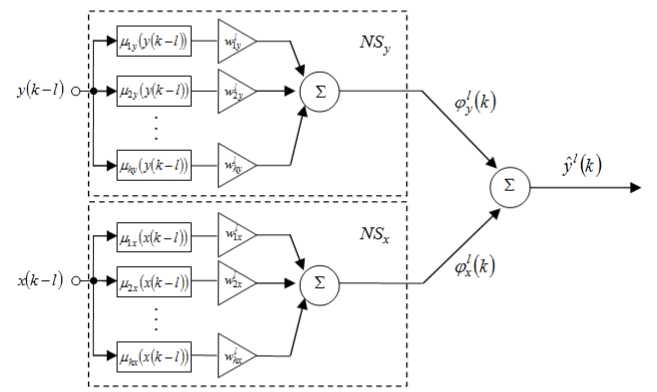
Fig.3. A neo-fuzzy node for the ANARX-model.

nh           h

y (k)=E|E w‘My (У (k -1))+X wx^ix (x(k -I))l,

- = 1 V i = 1                                 i = 1                           )

which means that since the neo-fuzzy neuron is also an additive model [24], the ANARX-model based on the neo-fuzzy neurons is twice additive.

Triangular membership functions are usually used in the neo-fuzzy neuron. They meet the unity partitioning conditions hh

X ц ( y ( k - ¹ ) ) = 1, X ^ -x ( ^x ( ^k - ¹ ) ) = 1, = 1                                     i = 1

which make it possible to simplify the node’s architecture by excluding the normalization layer from it.

It was proposed to use B-splines as membership functions for the neo-fuzzy neuron [25]. They provide a higher approximation quality and also meet the unity partitioning conditions. A B-spline of the q - th order can be written down:

1,if c-y  1 ci+q, y    ci+1, y i = 1,..., h - q,

1, if c^ <  x ( к - l )

0 otherwise

for q = 1

M ix ( x ( k ^{- l} ) ) = <

x P^ M ix - ( x ( к - 1 ) ) c i + q - 1, x    cix

-⁺ q ' ^x   x ⁽ k l ) M i - 1 x ( x ( к - 1 ) ) , for q >  1

ci+q, x    ci+1, x i = 1,..., h - q.

It should be mentioned that B-splines are a sort of generalized membership functions: when q = 2 one gets traditional triangular membership functions; when q = 4 one gets cubic splines, etc.

Introducing      a      vector      of      variables

^ ( ^к ) = ( M 1 y ( y ( ^{к - l} ) ) ^,...^, M hy ( y ( ^{к - l} ) ) ^, M 1 x ( ^x ( ^{к - l} ) ) ^,...^, M hx ( x ( ^{k -} l ^ ^{, W} = ( w ly ^,...^, w hy ^, w lx ^,...^, w hx ) ^{T , the} expression (5) can be rewritten in the form

y 1 ( k ) = wlT ^‘ ( к ) .

Either the algorithms (3), (4) or the procedure [26]

< w (к) = w (к -1)+r1 (к)(y (k) - wT (k -1)^ (k))^' (k)

Г (к) = art (к -1) + ^lT (к )фг (к), 0 < a < 1, can be used for the neo-fuzzy neuron’s learning. This procedure possesses both filtering and tracking properties. It should also be noticed that when a = 1 the equation (6) coincides completely with the Kaczmarz–Widrow– Hoff optimal algorithm (4).

Evolving systems based on the neo-fuzzy neurons demonstrated its effectiveness for solving different tasks (especially forecasting tasks [25-30]). The twice additive system is the most appropriate choice for data processing in Data Stream Mining tasks [11] from a view point of implementation simplicity and a processing speed.

• IV.    A W EIGHTED N EURO -N EO -F UZZY -ANARX-M ODEL

Considering that every node N ^{[ l ]} of the ANARX-model is tuned independently from each other and represents an individual neuro(neo)-fuzzy system, it is possible to use a combination of neural networks’ ensembles [31] in order to improve a forecasting quality. This approach results in an architecture of a weighted neuro-neo-fuzzy-ANARX-model (Fig.4).

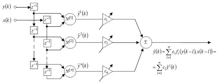
Fig.4. The weighted ANARX-model

An output signal of the system can be written in the form

n

y (к) = ZClyl (к) = cTy (к) l=1

where ^y ( к ) = ( y ( к ) ^{, y 2} ( к ) ^, ... ^{, y} n ( ^к ) ) , c = ( c ₁ ^, c ₂'...' c_n ) ^T is a vector of adjusted weight coefficients that define proximity of the signals y l ( к ) to the forecasted process y ( к ) and meet the unbiasedness condition

Z c l = c ^T I n = 1 l = 1

where I_n is a ( n x 1 ) -vector of unities.

The method of undetermined Lagrange multipliers can be used for finding the vector с in a batch mode. So, a sequence of forecasting errors

V(к) = y(к)-y(к) = y(к)-c ■y(к) = c Iny(к)-c y(к) = Iny(к)-y(к)) = c V(к), the Lagrange function

L(c,X) = EcTV(k)VT (k)c + X(cTI- -1) = k                                              (7)

= cT Rc + X( cT In -1)

(here X is an undetermined Lagrange multiplier,

R = E V(k) VT (k) stands for an error correlation matrix) k and the Karush–Kuhn–Tucker system of equations

c (k) = c (k -1) + n (k )x

^x ( ² ( y ( ^k )^{- c T} ( ^{k -} 1 ) ^y ( ^k ) ) y ( ^k )^{- X} ( ^{k -} 1 ) I n ) =

= c(k-1) + n (k)(2V(k)У(k)-X(k -1)In),

X(k) = X(k -1) + n (k)(cT (k)In -1)

\ _c L ( c , X ) = 2 Rc + X I„ = 0,

S L _ T r

.XX ~   "

- 1 = 0

are introduced. A solution of the system (8) can be written down in the form c = R-1 In (IT R-1 In )4, <

X = - 2 1 T R ^{- 1} I

where a value of the Lagrange function (7) at the saddle point is

L * ( c , X ) = ( I T R ^{- 1} I n )^{- 1}.

An implementation procedure of the algorithm (9) can meet some problems in a case of data processing in an online mode and a high level of correlation between the signals y l ( k ) that leads to the ill-conditioned matrix R which has to be inverted at every time step k .

The Lagrange function (7) can be written down in the form

L (c, X)=E( y (k)-cTy (k)) + X(cT In- 1) k and a gradient algorithm for finding its saddle point based on the Arrow–Hurwicz procedure [27, 32] can be written in the form c (k) = c (k -1)- nc (k )VCL (c, X),

/ _x             x       / x d L ( c , X )

X(k ) = X(k -1) + nX (k )   ■■ where n (k) and n (k) are learning rate parameters.

The Arrow–Hurwicz procedure converges to the saddle point with rather general assumptions on the values n ( k ) , n ( k ) , but these parameters can be optimized to speed up the learning process as that is particularly important in Data Stream Mining tasks.

That’s why the first ratio in the equation (10) should be multiplied by "y ^T ( k )

y (k) c (k ) = y c (k -1) +

+nc (к)l 2v(k)||y(k)|| -X(к- 1)y In and an additional function that characterizes a criterial convergence is introduced

(y(k)-yT (k)c(k)) = v2 (k)-

• ^{- 2} n c ( ^k ) v ( ^k ) ^ ² v ( k )||. y ( ^k )|| ^{- X} ( k ^- 1 ) ^{y T} I n ^) ⁺ .

+n2 (k)f2v(k)||y(k)||2 -X(k-1)yTIn)

A solution for the differential equation

^d ( y ( k )^{- y T} ( k ) c ( k ) )

d4c (k)

-2v(k)^2v(k)||y (k)|| - X(k -1)yTIn ^ +

+24c (k)[2v(k)||y(k)||2 -X(k-1)yTIn) = 0

or

gives the optimal learning rate values n _c ( k ) in the form

П с ( k ) =

_____________ v ^{( k} ) _____________

• 2 v ( k )||y ( k )|| - Я( k - 1) y T In

Applying this value to the expression (10), final equations can be written down

v(к)(2 v(к) y(к)-Л( к-1) In) c(k) = c(k - 1)+----^—^--------:—,

‘                      2v(k)||y(k)|| - Л(k - 1)yTIn

^(k) = A(k - 1) + n, (k)(cT (k)In -1).

It’s easy to notice that when Л ( k - 1 ) = 0 the procedure (11) coincides with the Kaczmarz–Widrow– Hoff algorithm (4).

• V.    E XPERIMENTS

In order to prove the effectiveness of the proposed system, a number of experiments should be carried out.

• A.    Electricity Demand

  This data set describes 15 minutes averaged values of power demand in 1997 (a full year). Generally speaking, this data set contains 15000 points but we took only 5000 points for the experiment. 3000 points were selected for a training stage and 2000 points were used for testing. Prediction results of the ANARX and weighted ANARX systems are in Fig.5 and Fig.6 correspondingly (signal values are marked with a blue color; prediction values are marked with a magenta color; and prediction errors are marked with a grey line).

We used for comparison multilayer perceptrons (MLPs), radial-basis function neural networks (RBFNs), ANFIS and two proposed systems ANARX and weighted ANARX (both based on neo-fuzzy nodes). The comparison of the systems ’ results is shown in Table 1. Since MLP can’t work in an online mode, it was processing data in two different modes. It had just one epoch in the first case (something similar to an online case), and it had 5 epochs in the second case (the MLP architecture had almost the same number of adjustable parameters when compared to the proposed systems). A number of MLP inputs was equal to 4 and a number of hidden nodes was equal to 7 in both cases. A total number of parameters to be tuned was 43 in both modes. It took about two times more time to compute a result in the second case but a prediction quality was like almost two times higher. MLP (case 2) demonstrated the best result in this experiment.

Speaking of RBFNs, there are two cases. The first-case RBFN was taken really close in the sense of para meters ’ number to our systems and the second-case RBFN’s architecture was chosen to show the best performance. In the first case, RBFN had 3 inputs and 7 kernel functions. In the second case, it had 3 inputs as well but 12 kernel functions which generally led to the higher prediction quality (+30% precision compared to RBFN in the first case) but took longer to compute the result. A number of parameters to be tuned was 36 in the first case and 61 in the second case.

ANFIS showed one of the best prediction qualities in this experiment. It had 4 inputs, 55 nodes and it was processing data during 5 epochs. It contained 80 parameters to be tuned.

Table 1. Comparison of the systems’ results

Systems	Parameters to be tuned	RMSE (training)	RMSE (test)	Time, s
MLP (case 1)	43	0.0600	0.0700	0.4063
MLP (case 2)	43	0.0245	0.0381	0.9219
RBFN (case 1)	36	0.0681	0.0832	0.6562
RBFN (case 2)	61	0.0463	0.0604	1.0250
ANFIS	80	0.0237	0.0396	0.7031
ANARX (neo-fuzzy nodes)	37	0.0903	0.0922	0.4300
Weighted ANARX (neo-fuzzy nodes)	36	0.0427	0.0573	0.3750

The proposed ANARX system based on the neo-fuzzy nodes had 2 inputs, 2 nodes, 9 membership functions, and its a parameter was equal to 0.62. This system had 37 parameters. Its prediction quality was rather high and it was definitely one of the fastest system on this data set. We should also notice that we used B-splines (q=2, which means that we used triangular membership functions) as membership functions for the proposed systems.

The proposed weighted ANARX system based on the neo-fuzzy nodes had 2 inputs, 2 nodes, 8 membership functions; its a parameter was equal to 0.9. It had 37 adjustable parameters. This system demonstrated better performance when compared to ANARX and the fastest results.

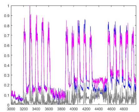
Fig.5. Identification of a nonlinear system. Prediction results of the ANARX system.

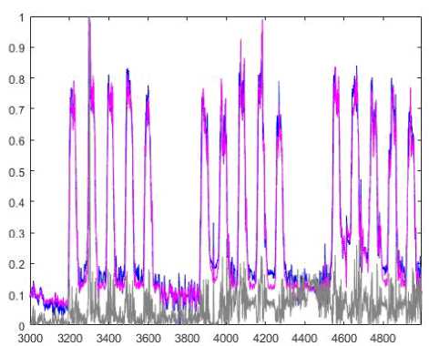
Fig.6. Identification of a nonlinear system. Prediction results of the weighted ANARX system.

ANARX and one of the fastest results.

Table 2. Comparison of the systems’ results

Systems	Parameters to be tuned	RMSE (training)	RMSE (test)	Time, s
MLP (case 1)	31	0.1058	0.1407	0.2813
MLP (case 2)	31	0.0600	0.0808	0.5938
RBFN (case 1)	21	0.1066	0.2155	0.2219
RBFN (case 2)	96	0.0702	0.1638	0.9156
ANFIS	80	0.0559	0.1965	0.8906
ANARX (neo-fuzzy nodes)	17	0.1297	0.1350	0.2252
Weighted ANARX (neo-fuzzy nodes)	20	0.0784	0.1081	0.2981

• B.    Monthly sunspot number

  This data set was taken from datamarket.com. The data set describes monthly sunspot number in Zurich. It was collected between 1749 and 1983. It contains 2820 points. 2256 points were selected for a training stage and 564 points were used for testing. Prediction results of the ANARX and weighted ANARX systems are in Fig.7 and Fig.8 correspondingly (signal values are marked with a blue color; prediction values are marked with a magenta color; and prediction errors are marked with a grey line).

We used a set of systems which is similar to the previous experiment to compare results. The comparison of the systems’ results is shown in Table 2. MLP_1 (MLP for the first case) had 3 inputs, 6 hidden nodes and it was processing data during just one epoch. MLP_2 basically had the same parameter settings except the fact that it was processing data during 5 epochs. Both MLP systems had 31 parameters to be tuned. MLP_1 was 2 times faster than MLP_2 but its prediction quality was also almost 2 times worse.

Let’s denote our RBFN architectures as RBFN_1 (RBFN for the first case) and RBFN_2 (RBFN for the second case). Both of them had 3 inputs. RBFN_1 had 4 kernel functions unlike RBFN_2 which had 19 hidden nodes. A number of parameters to be tuned was 21 in the first case and 96 in the second case. RBFN_2 showed a better prediction quality but it was much slower than RBFN_1.

ANFIS had 4 inputs and 55 nodes. It was processing data during 3 epochs. It had 80 adjustable parameters.

The proposed ANARX system based on the neo-fuzzy nodes had 2 inputs, 2 nodes, 4 membership functions, and its α parameter was equal to 0.9. This system contained 17 parameters. Its prediction quality was rather high and it was definitely one of the fastest systems on this data set.

The proposed weighted ANARX system based on the neo-fuzzy nodes had 2 inputs, 2 nodes, 4 membership functions; its α parameter was equal to 0.9. This system contained 20 parameters to be tuned. This system demonstrated better performance when compared to

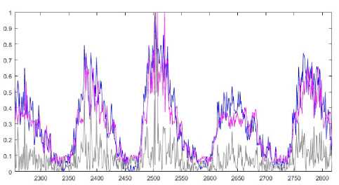
Fig.7. Identification of a nonlinear system. Prediction results of the ANARX system.

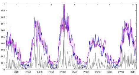
Fig.8. Identification of a nonlinear system. Prediction results of the weighted ANARX system.

• VI.    C ONCLUSION

The evolving forecasting weighted neuro-neo-fuzzy-twice additive model and its learning procedures are proposed in the paper. This system can be used for non-stationary nonlinear stochastic and chaotic time series ’ forecasting where time series are processed in an online mode under the parametric and structural uncertainty. The proposed weighted ANARX-model is rather simple from a computational point of view and provides fast data stream processing in an online mode.

So, the proposed evolving forecasting model has demonstrated its efficiency for solving real-world tasks. A number of experiments has been performed to show high efficiency of the proposed neuro-neo-fuzzy system.

A CKNOWLEDGMENT

The authors would like to thank anonymous reviewers for their careful reading of this paper and for their helpful comments.

This scientific work was supported by RAMECS and CCNU16A02015.