Adaptive Inverse Model of Nonlinear Systems

Published Online April 2015 in MECS

In many engineering applications, the system (plant) is nonlinear in characteristic. A sensor/actuator is nonlinear when it is operated beyond its operating range [1-4]. The communication channels are often nonlinear which demand a nonlinear channel equalization to get reduced bit-error-rate [5-7]. Optical communication system also has nonlinear distortion due to the nonlinear characteristics of the laser diodes, which needs to be compensated in order to enhance the performance [8-10]. A typical control system with a nonlinear plant needs linearization for performance improvement [11-15]. In active noise control, the nonlinear secondary path needs linearization for effective noise control [16-20]. In many cases the inverse model to the nonlinear transfer function (the physical system) is found out offline or periodically and placed at suitable location in the control/monitoring system to nullify the nonlinear effect of the system. Different types of nonlinear inverse models have been proposed for different applications. The nonlinear inverse model of a sensor using artificial neural network is proposed for pressure sensors [1]. To linearize the sensor model, subtle circuits are designed using simple and compact multiplier/divider and vector multiplier circuits that comprise of op-amps and MOS transistors [2]. Nonlinear compensation algorithms for extending the linear range of linear variable differential transformer are proposed in [3-4]. A number of nonlinear channel equalization algorithms are proposed which includes

Kalman filter-trained recurrent neural equalizers [5], radial basis function networks [6], artificial neural network trained by particle swarm optimization [7]. A higher order adaptive filter based predistortion system is used to compensate the nonlinear effect of fiber links [9]. In [11], an adaptive finite impulse response (FIR) filter based controller has been proposed for the tracking of a ferric ball under the influence of magnetic force. This adaptive filter is adapted to model the inverse system. Neural network based inverse model of nonlinear plants have been proposed for control applications [12-13]. A position control system has been proposed in [14] using an inverse model. The functional link artificial neural network is applied to find the inverse kinematics to control a robotic manipulator [15]. Active noise control (ANC) is a process by which antinoise is generated by a loudspeaker system to control the noise using principle of destructive interference. The loudspeaker system is a nonlinear system when it is driven beyond its dynamic range. In [16], usage of inverse model of the secondary path is used for better noise cancellation and sound reproduction. A linear equivalent of nonlinear inverse at every time instant is evaluated using a derivative method to find a time varying inverse model of the nonlinear secondary path for ANC application [17]. The same method is applied with advanced control architectures for nonlinear secondary path in [18-19]. An adjoint method to compensate the effect of linear secondary path is proposed for virtual active noise control [20]. The nonlinear systems can be static or dynamic. It can also be recursive. The physical nonlinear systems are modeled using either continuous or discrete equations. The nonlinear system models are realized as Wiener or Hammerstein types. These nonlinear systems may be time invariant or time varying. For linearization, an inverse model can be placed either before the plant (nonlinear system) or after the plant. When it is placed before the plant, it is called predistorter and when it is placed after the plant, it is called postdistorter. In a control application, mostly predistorter type inverse models are used, whereas for sensor and communication systems where the input is a physical quantity and the output is an electrical signal, the postdistorter type inverse model is preferred. In this case, the inverse model is followed by the nonlinear system or plant.

In summary, such nonlinear inverse models can be offline identified by using a nonlinear structure and a parameter optimization algorithm. The most popular nonlinear structure is a neural network and its variants. The optimization algorithms such as LMS and evolutionary computing algorithms are also used. The neural network architecture is a complex network and involves more computational complexity. The parameter update algorithm is also computationally intensive in this case. Therefore, in this paper, a simple adaptive algorithm is proposed for finding the nonlinear inverse of a nonlinear plant where the plant follows the nonlinear inverse model so that the over-all response is linear. The proposed filterbank based algorithm is simple to implement compared to the multilayer neural network algorithm.

Organization of this paper is as follows. Section II presents models of different types of nonlinear systems. A filter bank based nonlinear adaptive algorithm is proposed in Section III, for adaptively finding the inverse of a nonlinear system. Section IV deals with the simulation experiments to evaluate the performance of the proposed algorithms. Section V presents the conclusion.

• II.    Nonlinear Systems

Different types of nonlinear systems exist. In some systems the input is a physical quantity and the output is an electrical signal and in others, the input is an electrical signal and output is a physical quantity. There are systems where both input and outputs are either physical or electrical signals. The physical systems are generally continuous and to use digital signal processing, the input and output of the systems are discretized by analog to digital converters and may be represented in a discrete domain with a sample index n . Different types of systems and the mathematical relationship of the output of the system y ( n ) with the input of the system x ( n ) is presented below.

• A.    Static nonlinear system

The system whose output is a nonlinear function of the present input only and is represented as y (и ) = f (x (и»,                                   (1)

where n represents the sample time index, f (.) is the nonlinear function. x ( n ) and y ( n ) are the input and output of the system, respectively. Many practical systems and sensors have static nonlinearity. The block diagram of a static nonlinear system is shown in Fig. 1 (a)

• B.    Dyanamic nonlinear system

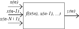
Dynamic nonlinear system: The system whose output is a nonlinear function of the present and past inputs and is represented as [21]

y ( и ) = f ( x ( и ) x ( и - 1),..., x ( и — N + 1)).             (2)

The output of a dynamic system may also depend on the past outputs which is also called as recursive system and is represented as

y ( и ) = f ( x ( и ), x ( и - 1),..., x ( и - N + 1),

y ( и - 1), y ( и - 2),..., y ( и - M + 1)).                   (3)

The dynamic nonlinear systems may be modelled as a linear combination of nonlinear functions of present and past inputs and past outputs and are represented as

y(и ) = fо(x(и))+f(x(и -1)),..., fN-1(x(и - N+1», g1(y(и -DX g2(y(и - 2)),..., g3(y(и -M +1))       (4)

The block diagram of a dynamic nonlinear system is presented in Fig. 1 (b).

• C.    Cascade system

The static and dynamic nonlinear system may be cascaded with a linear system to form another type of nonlinear system. A physical system may have a linear part and nonlinear part. The system when excited by certain range of input signal may behave linearly and beyond this range it becomes nonlinear. In literature [22] two such system are well studied: Wiener and Hammerstein.

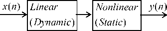
The Wiener system is also called as Linear-Nonlinear (LN) system, where a static nonlinear model is followed by a dynamic linear system. This is expressed as

_Z ( и ) = ] - 1 h_kx ( и - k )                                  (5)

k = 0

y ^{( и} ) = ^{f (} z ^{( и})) ,                                      ⁽⁶⁾

where z ( n ) is the output of the linear dynamic system represented here as a finite impulse response (FIR) filter and f (.) is a static nonlinear function operates on the output of the linear system to generate the output of the Wiener system. The block diagram of a Wiener system is shown in Fig. 1 (c).

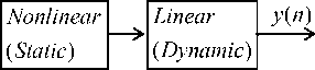
The Hammerstein system is also called as Nonlinear-Linear (NL) system, where a static nonlinear model follows a dynamic linear system. This is expressed as

z ^{( и} ) = ^{f ( x ( и}))                                       ⁽⁷⁾

N - 1

y ^{( и} ) = Z h k z ^{( и - k} ),                              ⁽⁸⁾

k = 0

where z ( n ) is the output of the static nonlinear system which is fed to a finite impulse response (FIR) filter to generate the output of the Hammerstein system. The block diagram of a Hammerstein system is shown in Fig. 1 (d).

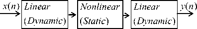
A Wiener system can be concatenated with a Hammerstein system to generate a structure which is equivalent to linear-nonlinear-linear (LNL) combination of systems. The block diagram of a LNL system is shown in Fig. 1 (e).

x(n)             y(n)

f(x(n))

(a)Static nonlinear System

(b)Dynamic nonlinear System

(c) Wiener system (LN System)

(d) Hammerstein system (NL System)

(e) LNL system

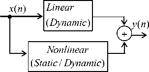
(f) LN Parallel System

Fig. 1. Schematic diagram of different system

In addition to this, these static nonlinear systems may be dynamic based on the nonlinear phenomena in a physical system.

• D.    Parallel system

Unlike the cascaded systems, where the linear and nonlinear systems are combined in series, they can be combined in parallel. If the input of a system sees both nonlinear and linear effects on its path, till it reaches the output. The block diagram of a parallel system is shown in Fig. 1 (f).

• III.    Proposed Algorithm for Estimating Nonlinear Inverse Model

The linear adaptive filter consists of a finite impulse response (FIR) filter which is excited by a direct input signal. The coefficient of this adaptive FIR filter is updated using some adaptive algorithms such as least mean square (LMS) algorithm. However, these linear adaptive filters are not suitable for finding the inverse of a nonlinear system.

In case of a nonlinear adaptive filter, a bank of parallel FIR filters is present. Each of these filters in the filter bank are excited by the nonlinearity modulated input signal. In other words, the input signal x(n) can be represented as, yif (n) ∈{y(n), sin(πy(n)), cos(πy(n)),..., sin(Pπy(n)), cos(Pπy(n)) }(9)

This is also termed as FLANN based algorithm [23-27]. Using power series, the x(n) is expanded as, yif (n) ∈{y(n), y2(n), y3(n), y4(n),...,yM(n)}(10)

Using a second order Volterra series the x(n) expanded as, yif (n) ∈{y(n), y2(n), y(n) y(n-1), y(n) y(n-2),…,

y(n)y(n-N+1) }(11)

Each of these elements of the functionally expanded element of the above series y^f ( n ) acts as an input of an individual FIR filter. Since these series are created by nonlinear functions operated on y ( n ) and are input to individual filter, such a structure is named as a nonlinear adaptive filter. The outputs of each of these adaptive filters are summed up to generate the output of the nonlinear adaptive filter x ˆ( n ).

MN - 1

x ˆ( n ) = ∑∑ y_i^f ( n - j ) h_{i , j} ( n ).                      (12)

i = 1 j = 0

Here right hand side summation is a convolution operation which represents the filtering operation. N represents the length of these filters which is either fixed for every type of input or variable. The Volterra series expansion uses a variable order filters where as the trigonometric and the power series expansion uses a fixed order filters. M is the total number of functionally expanded coefficients. The adaptive structure of the proposed algorithm to model the inverse of a nonlinear system is presented in Fig. 2. The output of this model, x ˆ ( n ) is compared with a direct or delayed version of the actual excitation signal of the nonlinear plant, x ( n ) to get

e ( n ) = x ( n - ∆ ) - x ˆ( n ) .                           (13)

where Δ is an integer delay which can be 0, 1, …D. The D represents the overall delay of the nonlinear system and its inverse. D is nonzero when the nonlinear plant has some inherent delay. This delay Δ can be minimized only when the inverse model is estimated with a predictable input signal. The coefficients of these filters, h ( n )of the model of the inverse of the nonlinear system are updated using a least mean square (LMS) algorithm.

h _i ( n + 1) = h _i ( n ) + µ e ( n ) y _i ^f ( n )                     (14)

where    h _i ( n ) = { h_{i ,0}, h_{i ,1},..., h_{i , N - 1}}                     (15)

is the time varying coefficient vector of the i th filter and y f (n) is the corresponding input signal vector defined as yf (и) = {yf (n),yf (n-1),...,yf(n - N + 1)}. (16)

ц is the step-size parameter. This control structure can also be updated by other suitable algorithms such as recursive least square (RLS) and derivative free algorithms such as genetic algorithms and particle swarm optimization. The proposed algorithm assumes that there exists a suitable inverse model of the nonlinear plant and the inverse model has a nonlinear structure. Accordingly, the output of the nonlinear system is functionally expanded to most possible nonlinear operation to cope with the nonlinear inverse model requirement.

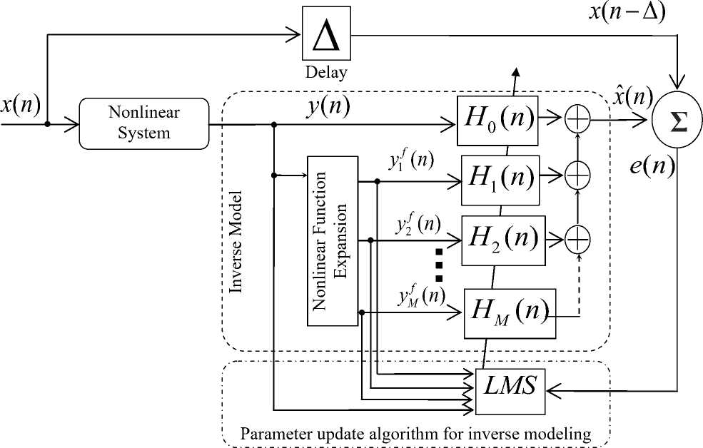
Fig. 2. Estimation of nonlinear inverse model using filter bank based nonlinear adaptive structure

• IV.    Simulation

To evaluate the performance of the proposed nonlinear inverse modeling algorithm, several nonlinear systems/plants are chosen. Both second order Volterra series presented in (12) and trigonometric series (FLANN) using series in (10) are simulated for each nonlinear system and the mean square errors in dB are plotted for both the algorithms.

• A.    S mulat on 1

Here the nonlinear system is chosen as y (n) = 0.5 x (n) + 0.1 x 2( n) + 0.3 x 3( n) - 0.5 x 4( n).    (17)

This is a static nonlinear system as the y(n) does not depend on any past values of x(n). This nonlinear system is excited by a random white noise generated between -0.5 to 0.5. The comparative convergence plot is shown in Fig. 3 where both second order Volterra series and trigonometric series (FLANN) based inverse models are simulated using LMS algorithm. Step size for Volterra and FLANN systems are chosen as 0.5 and 0.5 respectively. This figure shows that the FLANN based inverse model has superior performance compared to the second order Volterra based inverse model.

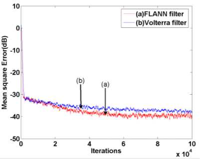
Fig. 3. Convergence characteristic of MSE for a static nonlinear system(Simulation-1)

• B.    Simulation 2

In this simulation, the nonlinear system is chosen as, y ( n ) = x ( n ) + 0.5 x ( n - 1) + 0.9 x ( n - 2)

- 0.5 x ( n ) x ( n - 1) + 0.4 x ( n ) x ( n - 2).

This is a dynamic nonlinear system as the y ( n ) depends on past value of x ( n ). This nonlinear system is excited by a random white noise generated between -1 to 1. The comparative convergence plot is shown in Fig. 4. Step size for Volterra and FLANN systems are chosen as 0.005 and 0.005 respectively. This figure shows that the Volterra based inverse model has slightly superior performance compared to the FLANN one. This is because the Volterra series involves cross terms and this nonlinear system possess cross terms.

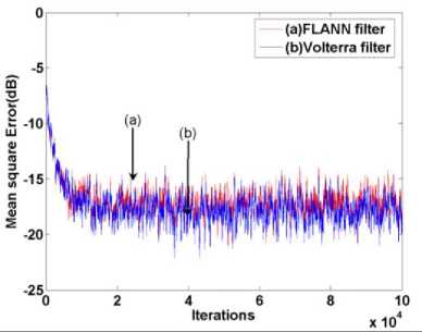
Fig. 4. Convergence characteristic of MSE for a dynamic nonlinear system(Simulation-2)

• C.    Simulation 3

Here the cascaded linear-nonlinear system is chosen as z (n) = x (n) - 0.6 x (n -1) + 0.05 x (n - 2)            (19)

FLANN systems are chosen as 0.05 and 0.05 respectively. From the figure it is seen that the FLANN filter outperforms the Volterra based system for inverse modeling.

• D.    Simulation 4

Here the cascade system is chosen as z (n) = tanh( x (n))                                   (21)

y ( n ) = z ( n ) + 0.2 z ( n - 1) + 0.5 z ( n - 2)              (22)

This is a Hammerstein system as the z ( n ) represents the output of the nonlinear part of the system and y ( n ) represents the output of the linear part. This nonlinear system is excited by a random white noise generated between -1 to 1. The comparative convergence plot is shown in Fig. 6. Step size for Volterra and FLANN systems chosen are same as in simulation-3. This figure show that the FLANN based inverse model and the second order Volterra based inverse model has the same performances.

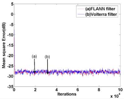
Fig. 6. Convergence characteristic of MSE for a Hammerstein system(Simulation-4)

y ( n ) = tanh( z ( n ))

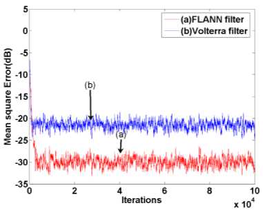
Fig. 5. Convergence characteristic of MSE for a Wiener system(Simulation-3)

This is a Wiener system as the z ( n ) represents linear part of the system and y ( n ) represents the nonlinear part. This nonlinear system is excited by a random white noise generated between -1 to 1. The comparative convergence plot is shown in Fig. 5. Step size for Volterra and

• E.    Simulation 5

Here the cascade system is chosen as z1( n) = x (n) - 0.6 x (n -1) + 0.5 x (n - 2)(23)

z 2( n ) = tanh(z1( n ))(24)

y (n) = z 2( n) + 0.2 z 2( n -1) + 0.5 z 2( n - 2)(25)

This is a LNL system as the z 1( n ) represents the output of first linear system and z 2( n ) represents the output of the static nonlinear part and y ( n ) represents the output of the final linear part. Therefore, this is an LNL system. This nonlinear system is excited by a random white noise generated between -1 to 1. The comparative convergence plot is shown in Fig. 7. Step size for Volterra and FLANN systems are chosen as 0.01 and 0.01 respectively. Here the convergence performances of both the algorithms are almost same.

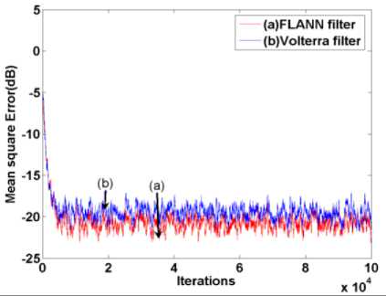
Fig. 7. Convergence characteristic of MSE for a LNL system(Simulation-5)

• F.    Simulation 6

Here the parallel system is chosen as z1( n) = x (n) - 0.6 x (n -1) + 0.5 x (n - 2)(26)

z 2( n) = tanh( x (n))(27)

y (n) = z1( n) + z 2( n)(28)

This is a parallel system as the z1(n) represents the output of the linear part of the system and z2(n) represents the output of the nonlinear part and y(n) represents the final output of the parallel combination of both of them. This nonlinear system is excited by a random white noise generated between -0.5 to 0.5. The comparative convergence plot is shown in Fig. 8. Step size for Volterra and FLANN systems are chosen as  0.005  and 0.05 respectively. Here also the performances of both the algorithms are almost same.

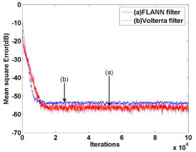
Fig. 8. Convergence characteristic of MSE for a LN system in parallel(Simulation-6)

• V. Conclusion

In many practical applications, the system is nonlinear and hence its control is difficult. These nonlinear systems can be linearized by placing its nonlinear inverse model either before or after the said system. This paper proposes a generalized filter bank implementation of nonlinear adaptive filter algorithm. This algorithm can use any nonlinear series expansions of a signal and can be suitably applied without any modification in the weight update algorithm. This algorithm is applied to estimate the nonlinear inverse of any nonlinear system to achieve overall linearization. The nonlinear system cascaded with this inverse model becomes linear and helps engineers to use suitable linear techniques.

In this paper, a number of synthetic plants were chosen for performance evaluation of the proposed algorithm used as an inverse model. It is found that FLANN and Volterra series based filters behave almost similarly in many cases. However, the second order Volterra filters has lower mean square error compared to FLANN filter when the nonlinear system have cross-terms. The FLANN achieves better performance under higher order nonlinearity cases. The proposed algorithms can be suitably applied in channel equalization, control, instrumentation and active noise control problems.

Acknowledgment

• P. Patnaik acknowledges CSIR-IMMT for permitting her to work for her M.E.(Computer Science and Engineering) thesis work.