Adaptive Observers for Linear Time-Varying Dynamic Objects with Uncertainty Estimation

Published Online June 2017 in MECS DOI: 10.5815/ijisa.2017.06.01

Construction of adaptive observers (AO) is one of the rapidly developing areas of control theory. The basis of theory AO for the linear class of dynamic systems has been obtained an the end of past century [1-6]. The class of adaptive systems having a special identification representation in space "input-output" was proposed. Despite this, the research in this area continues. In particular, design methods of AO for time-varying objects are proposed. The majority of the approaches are based on the generalization of the results which are obtained for linear time-invariant dynamic systems.

So, problem of combined identification and control of the discrete dynamic system with time-varying parameters is considered in [7]. It is supposed that parameters are piecewise constant, and the modification time is determined by means of the Markov chain. Convergence of adaptive algorithms is proved. The set of criteria allowing minimizing an error of forecasting an output system is applied to improve an efficiency of control. Such approach complicates identification systems. The problem of adaptive identification time-varying nonlinear plant is considered in [8]. It is supposed that the plant state vector is measured and description of a nonlinear part of the system is known. The unknown vector of system parameters approximates Taylor series. The adaptive algorithm of identification is offered. Lüders-Narendra adaptive observer is applied to stabilization of time-varying nonlinear continuous system in [9]. Boundedness of trajectories in an adaptive system is proved.

Methods of adaptive control dynamic systems with variable parameters are proposed in [10]. It is supposed that parameters have the restricted velocity of the change. Boundedness of trajectories in an adaptive system is proved. This approach improves the quality of transients in an adaptive system. It on nonlinear time-varying systems can be generalized.

A multidimensional linear time-varying dynamical system is considered in [11]. Matrixes of state and control are considered as the known functions of time. It is supposed that the linear part of the system depends on an unknown parameter vector. The adaptive Kalman filter for a state estimation and system parameters is offered.

Considered methods and algorithms do not allow ensuring the unbiasedness of obtained estimations [12, 13]. Explain it to that the law of the change parameters is unknown. Therefore, the majority of approaches on the qua-si-stationary hypothesis are based.

The solution of design problem AO can be based an application: (i) different methods of time-varying parameters approximation [8]; (ii) the compensating control influences [9, 14]. Choice of the reference model for AO in [14] is realized on the basis of the analysis the a priori information. The law of parameters objects change under the uncertainty is usually unknown. Therefore, the object as a system with parametric uncertainty is considered.

Adaptive observer application for the control of stationary uncertain objects is given in [3, 15]. The case when uncertainty is a discrepancy of a model to plant (structural disturbances) is studied. Such disturbances are called non-modeling dynamics. Algorithms which ensure robustness to these disturbances are designed.

So, the problem of time-varying systems identification is topical. The condition of the excitation constancy is the basis of the design effective adaptive systems. This condition often is not fulfilled. Stability AO under these conditions was not studied. The second important problem is the parametric disturbances estimation in a system. As a rule, parametric disturbances suppose the restricted. A posteriori method of the parametric uncertainty estimation was not offered.

We propose the method of design AO for a linear timevarying dynamic object at condition EC non-fulfillment. The problem of synthesis the adaptive observer is divided into two subtasks. The solution of the first problem gives a choice of the constant matrix alleviating condition EC. This matrix superimposes restrictions on the parameters vector AO. The method of the matrix construction is proposed. The set (vector) of multiplicative adjusted parameters (MAP) is introduced at the second stage of the problem solution. The method of the dimension choice MAP is proposed. Adaptive identification is reduced to the design problem of algorithms under restriction. The method ф -algorithms [15, 16] is applied to its solution. Next, the problem of uncertainty estimation in the object is considered. Two approaches are offered to the solution of this problem. The first approach allows obtaining static model on the basis which the uncertainty estimation is determined. The adjusted parameter is introduced for raise of an exactitude of the estimation. It allows minimizing a total the prediction error. The second approach is based on the construction of a static model depending on current values of parameters AO. We introduce the adjusted parameter. It raises the exactitude of the uncertainty estimation. Boundedness and exponential dissipativity of trajectories of the adaptive system are proved. Computer modeling AO is fulfilled.

The work has the following structure. Section 2 contains the problem statement. The equation AO is obtained in section 3. The control compensating uncertainty is introduced. Main assumptions concerning properties of the system are considered. Parametrization of the control for increase of identification accuracy is performed. The parametric variable allowing adapting control to the existing uncertainty is introduced. The design of adaptive algorithms at non-performance of excitation constancy condition is proposed in section 4. Multiplicative parameters are introduced for fulfillment EC in a special parametrical space. ф -algorithms of the parametrical variable tuning are designed. Variants of the accounting of a posteriori information on the system are c o nsidered. Section 5 gives the description of a matrix H choice ensuring contraction of parametrical space AO for fulfillment EC. The condition of dom i nation is algorithm basis for the design of the matrix H . The problem of the uncertainty estimation is considered in section 6. The task solution is based on the introduction of a variable estimating uncertainty in the system. The adjusted coefficient ll before this variable raises the estimation accuracy. Properties of the adaptive system are researched in section 7. Boundedness of adaptive system trajectories is proved. Properties of AO with various algorithms for control and adaptation are researched. Obtained results are based on the application of Lyapunov vector functions. The proof of main statements is given in appendices. Results of modeling are presented in section 8. The conclusion contains the short review of obtained results.

• II.    Problem Statement

Consider the object described by the equation

x ^{( m} ) + a_m(t ) x ^{( m} ) + ...+ a_x ( t ) x = b ( t ) r , y = x ,    (1)

where 0 (t ) = [ a ( t ) a ₂ ( t )... a_m ( t ) b (t ) J T , r e R , y e R are input and output, 0e G₆ , G_e c R^{m + 1} is restricted and a priori an unknown area.

Components of the vector , ( t ) have the form

, (t) = ^ + A, (t) , i = 1, m +1, where |a, (t)||<, = const > 0, ^ = const.

The laws of change , ( t ) also are unknown.

Assumption 1 . The change velocity A , ( t ) is restricted and unknown.

Assumption 2 . The vector A0 ( t ) = 0 ( t ) -0 ° belongs to set

A0e G , \G^,           (2)

where 0 ° = ^ a_x ° a ° ... a ° b ⁰ J .

• (2)    is the condition of uncertainty. The experimental information on an object has the form

Io ={r(t)>y(t) t e J} , where J c R is the specified interval of the time.

The condition EC is not fulfilled for the input r ( t ).

Problem: design for (1) adaptive observer that the condition was satisfied lim y(t)- y(t) < ny,(3)

where y ( t ) is output AO, n - °.

• III.    Equation of Adaptive Observer

Write the equation (1) in the form y = 0TP + f (y, r, A0),(4)

where P e R ^{2 m} is the generalized input representing an output of the auxiliary filter

P1 = [Л + Л] P1 + [iTylTr]T ,(5)

P = [ y P^T r P^T ] ^T , P = [ P^T P^T ] ^T , P ∈ R ^{2 m - 2} is the vector of auxiliary signals obtained on the basis of transformation r ( t ) and y ( t ); + is the sign of the direct sum of matrixes; Λ ∈ R^{m - 1} is the diagonal matrix with λ <  0 ( i = 1, m - 1 ) ; I ∈ R^{m - 1} is unit vector; Θ ∈ R ^{2 m} is a vector corresponding Θ ⁰ ; f ( y , r , ΔΘ ) ∈ R is a component depending on the parametric disturbance ΔΘ in (1).

Assumption 3. The input r ( t ) does not satisfy a condition of constant excitation.

Assumption 4. f ( y , r , ΔΘ ) <∞ at | r ( t ) | <∞ .

Apply to the object described by the equation (4), adaptive model [17]

y ˆ =- k ( y ˆ - y ) + N^TH^TP + u ,       (6)

where H ∈ R ^{2 m × l} is a matrix with constant parameters, N ∈ R^l is a vector of adjusted parameters, u ∈ R is a control, l < 2 m .

Present u ( t )in the form

u(t) =DT(t)P(t) ,(7)

where D ∈ R ^{2 m} is some restricted vector.

Write the vector D as

DT(t) = µ(t)D,(8)

where D ∈ R ^{2 m} , II D ( t ) II ≤ d , d >  0 is some number, µ ( t ) ∈ R is controlled variable.

We suppose that

µ(t)∈Gµ ={µ∈R:I µ(t) I≤1 ∀t≥t0}.(9)

The choice of the vector D ensures fulfillment of the condition (9).

• IV.    Design of Adaptive Algorithms

We propose an approach to the design of the adaptive observer at non-performance EC. The preliminary estimate H of parameter vector the object (4) is obtained. The multiplicative tuned vector N ( t ) at matrix H has introduced that fulfillment of conditions EC and (3) to ensure. Adaptive ϕ -algorithm for vector is obtained. It is based on the accounting of existing restrictions

Go to the design of adaptive algorithms for the vector N(t) and the variable µ(t). Write the equation for an identification error e(t) as e=-ke+NTHTP-ΘTP-f(y,u,ΔΘ)+µz,   (10)

where z = D^TP .

We see from (10) that the vector HN ( t ) should approximate unknown parameters vector of the object (4). As parametric uncertainty exists, e ( t ) cannot be reduced to zero. Apply control u ( t ) to ensure fulfillment of the condition (3).

Linearize function f ( ⋅ )

f ( y , u , ΔΘ , t ) =ΔΘ ^T ( t ) P ( t ) ,         (11)

where ΔΘ ( t ) is some vector.

We assume that on the basis of the made assumptions

| f ( y , u , ΔΘ , t )| ≤ ρ _f = const ≥ 0.       (12)

Choose dimension l the vector N ( t ) on the basis of frequency properties the input r ( t ) . Designate the approximation error Θ + ΔΘ ( t ) with the vector HN ( t ) as δ N ( t ):

δ ( t ) = HN ( t ) -Θ-ΔΘ ( t ) .

δ ( t ) satisfies (2) and depends on the parametric uncertainty of the object (4). Uncertainty depend from δ ( t ) and satisfies the condition (12). Therefore, the condition is true for Θ ^ˆ ( t ) = Θ+ ΔΘ ( t )

Θ ^ˆ( t ) ∈ G ^k A ⇔ α ˆ θ ≤ Θ ^ˆ( t ) ≤ α θ .

Then we have

II HN ( t ) II≤ α _N , α _N <∞ .

We obtain from δ ( t ) inequality

ν=αN -αθ≤ δN(t)≤ αN -αˆθI=ν1.(13)

Then the vector N ( t ) at a corresponding choice of matrix H belongs to set

N∈GN={N∈Rl: ni(t)I ≤1 i=1,l }.(14)

Write (11) as e = -ke+δTP+µz .(15)

Transform the equation (15) to the form e = -ke+σTP-σTP+µz, where aN(t) = HN(t)-0, ^ = A0(t) . Let h^ = ^TP .

Apply the method ф -algorithms [15, 16] to the design of adaptation algorithms. Consider Lyapunov function V_e (t ) = 0.5 e ²( t ) . F- form is true for the derivative X ( t ) = V e ( t )

X = - ke ² I T N ( N ) Ф N ( e , N , H , F ) + e _CT ^T T F + e ^ z , (16)

Where

Ф N = eF ( I T D (I N ) I ) ^{- 1} ^ N , T N ( N ) = I T D (I N ) I ,

|N | is the absolute value of the vector N ( t ), D (| N |) is diagonal matrix from the vector N , I e R^l is the unit vector.

Obtain from (16) ф -algorithm for adaptation the vector N ( t )

N = - e r p ( N ) H T F ,        (17)

where Г e R^{l x l} is a symmetrical positive-definite matrix, P ( N ) is a belonging matrix indicator N e G _x .

Various methods of the definition P ( N ) are applicable.

If the indicator P (N)to present in the form f I, N (t) e Gn

P ( N ) =    ^l’         ^N

[ 0,, N(t) g G„ that multiplicative ф -algorithm for N(t) has the form

^ = I-erHTF, N(t) e Gn , [     01, N (t) g G n , where It, 0Z unit and zero matrixes l x l.

Matrix H for accuracy raise can be computed on each interval of a quasi-stationary object.

Design the control law for the variable a(t). Let conditions (8), (9) are satisfied. Determine the adjustment law a(t) from the condition min max V (n, SN, t) .(19)

n    Sn   eN max V(t) on SN (t) is obtained on domain boundary (13), that is at such value SN (t), when ||Sv (t)||=4 • Therefore, transform x(e, A, t) to form

X - -ke2 + Tц (e, A, z) Фa (e, A, z) + |e| ||Sn|| IIPII, where Тд = |e||DTF|, Ф^ = Asgn(e)sgn(DTF).

As a e G^ the adaptive observer is robust to uncertainty ^h A = F T ^F , ^if

||D|| > c(V1),(21)

where c ( v ) >  0 is some number.

Obtain the following tuning ф -algorithms of the variable a ( t ) on the basis (20) and (19):

• i)    static Μ -algorithm

A(t) = -Ys sgn(e(t)) sgn(DTF(t));(22)

• ii)    dynamic Μ -algorithm

A( t) = -Ya, sp(A)sgn (e( t)) sgn (DT F(t));

• iii)    dynamic Μ - algorithm

A(t ) = -Ya P (A) e (t) DTF(t),(24)

where P ( a ) is the belonging indicator a ( t ) e G^ , Y s >  ⁰, Y a >  ⁰, Y a , s >  ^0.

Other algorithms for a ( t ) can be obtained from the condition x - 0 .

• V. Choice of Matrix H

Consider the equation (4). Apply the operation of the differentiation to determination y . Designate the obtained variable as y_d (t ). Choose time gap J_d c J the change y so that system properties on it were homogeneous. It means that the trajectory y ( t ), and, hence, y ( t ) should not have structural modifications.

Consider on the interval J the equation

Уа = HTF, where H e R2 m, H = HI, I e R2 m.

Apply the least-squares method and obtain the vector H as the problem solution min (y - ya )2 ^ H.

H

Demands to the estimation H .

H1. H ensures the following condition of dominance

У(t)  Уа (t) for almost Vt e J c J, where J contains all t, since some t > 4 > t0.

H2. Elements of vector H ensure the performance of the adaptive system.

Condition H2 is very important, as tuning of vector N ( t ) in (6) depends on the elements of the vector H . As l <  2 m we consider only such estimations N ( t ) which ensure minimization of functional

Q ( N ) = ( H ( H ) N ( t ) -0 ) 2 .

Remark 1. The estimation H is obtained from the quasi-stationary condition of change system parameters. This estimation has the approached character, sufficient for implementation of the adaptive system.

Remark 2. If traj e ctories of the adaptive system are not restricted the set H , fulfill one of following operations.

• 1.    Obtain the estimation H for t e J^ , where J _M # J * .

• 2.    Change dimension l of the vector N ( t ). It will lead to the replacement of the vector H by the matrix H .

• VI.    Uncertainty Estimation

Obtaining D in the conditions of uncertainty is the complicated problem. Therefore, apply the following approach. It is based on obtaining of a variable for the estimation h ( t ).

Construct model

У d = H J P               (25)

for prediction of the variable y ( t ), and compute values of the error s_d (t ) = y ^ ( t ) - y_d (t ) . s_d ( t ) is the uncertainty estimation in the system.

Remark 3. We have introduced the vector H to distinguish it from the vector H used for the formation of the matrix H in model (6).

Present model (6) and the equation for the identification error (15) in the form

SED : У = - k ( y - y ) + N T H T P + p_£^ , e = - ke + r T P + g_d ,                (26)

Me = -Yse^d, where gd = иуу -oTP, lu is the adjusted parameter.

p adjusted level ^ that of disturbance effect to compensate in the adaptive system. Disturbances are a result of the application the model y^ = H T P and the action h д ( t ) .

Remark 4. Demands to the vector H considered in section 5 should be considered, when the variable ^ ( t ) is determined.

Another approach is based on obtaining of the uncertainty estimations on the basis of current adaptation results use. Apply model yd, N = NT HTP,             (27)

and determine the error ^ ( t ) = y ^ ^( t ) - y_d (t ) . ^ is the current estimation of the uncertainty h ( t ).

Use of the model (27) complicates the adaptation process. But work quality of adaptive system under some conditions improves at the application of the model (27). Here dimension of the vector N ( t ) has the significant effect. Therefore, the compromise necessary to observe between dimension of the vector N ( t ) and properties I .

Write the model (6) and the equation for identification error (15) for the case (27) as

SEN : y = - k ( y - y ) + N T H T P + p^ , e = - ke + ^NP + g N ,                 (28)

Pn = -7Ne£N, where gN = pNeN - a^P, p is the tuned parameter.

• VII.    Properties of Adaptive Systems

Consider properties of the adaptive system AS^ss which is described by equations (7), (8), (15), (17), (22). Boundedness of trajectories follows from the following assertion.

Theorem 1. Let conditions are satisfied: 1) function Ve (t) = 0,5e2 (t) is positive definite and satisfies the condition inf V (e, t) ^ ^ ; 2) assumptions 1, 2 for the ob-| e| ^да ject (1) are fulfilled; 3) the parameter N(t), p(t) of the model (6) belong to restricted areas G , G . Then all trajectories of system ASss are restricted and fair estimations

t

J ( 2V_e ( r ) - Y s ^ 4 2 V e ( r ) ) d r <  V ( t о ) - V ( t ), t ₀

^V e ^{( t} ) <    I ^ P maxl I ⁵ " ⁽ t )ll ⁺ Y s ^U z I ,      ⁽²⁹⁾

t where д = min |^TP|, uP = max||P(t)||2, и = max|z(t)|,

• V ( t ) = V e ( t ) + ∫ δ N ^T ( τ ) Γ^{- 1} Ψ N ( N ) δ N ( τ ) d τ .   (30)

t ₀

The proof of theorem 1 is given in Appendix A.

The theorem 1 shows that all trajectories of the adaptive system AS^ss are restricted. Limiting properties AS^ss -systems depend on the work of the adaptive algorithm (17) and the control law (22) variable µ ( t ). Μ -algorithm ensures fulfillment of the condition (3). The decrease of the error e ( t ) depends on the choice of the parameter γ Μ -algorithm.

Consider AS^ds -system described by equations (7), (8), (15), (17) and (23).

Theorem 2. Let conditions of the theorem 1 are satisfied. Then all trajectories of the system AS^ds are restricted and fair estimations (29) with γ ² = 1 , and

t

∫ 2 V e ( τ ) d τ ≤ V ( t 0 ) - V ( t ). t ₀

So, Μ , Μ -algorithms ensure fulfillment of the target condition (3). Specific properties of algorithms do not allow improving the quality of the adaptive system work.

The proof of theorem 2 is given in Appendix B.

Consider AS^d -system described by the equations (7), (8), (15), (17) and (24).

Theorem 3. Let conditions of the theorem 1 are satisfied. Then all trajectories of the system AS^d are restricted and fair the estimation

V_e ( t ) ≤ υ ^P ₂ max δ _N ( t )II2_.

The proof of theorem 3 is given in Appendix C.

We see that the condition (3) with π = 0 in ASd -y            Nµ system can satisfy. It is possible if the vector HP(t) is constantly excited.

Consider properties of the algorithm (18). The equation for an error writes in the form e = -ke+σTP-σTP+µz,        (31)

where

σ N ( t ) = H ( N ( t ) - N Θ ) = H Δ N ( t ), Θ= HN , σ = ΔΘ ( t ).

Definition 1   [18]. The non-positive quadratic form

W ( Y , X ) has M -property or W ( Y , X ) ∈ M , if it is representable as

W(Y,X)=-cyIIY II2 +cxyWxy(Y,X), for any Y∈ Rm , X∈ Rn in limited area

Ω ={Y∈Rm,X ∈RnIIIY II2+ X 2≤α, α≥0}, where IIY II is Euclidean norm of a vector Y , c > 0 , c ≥ 0 , W (Y,X) is some function.

Definition 2 [18]. The non-positive quadratic form

W ( Y , X ) has M ⁺ -property or W ( Y , X ) ∈ M ⁺ , if it is representable as

W(Y,X)=-cyY2+cxX 2, for any Y∈ Rm , X∈ Rn in the restricted area Ω , where cx ≥ 0.

M ⁺ -property is an indication of a constructive completeness of the quadratic form W ( Y , X ) . It allows reducing the analysis of properties W ( Y , X ) to an estimation of characteristics corresponding M -matrix [19].

Definition 3. The vector P ( t ) = H^T P ( t ) , P ∈ R^l is constantly excited with level α or has property PE , if

PEα: PH(t)PHT(t)≥αIl for some α > 0 and ∀t≥t on some interval T > 0 .

The system (1) is stable, and the input r ( t ) is restricted. Therefore, property PE for the matrix B ( t ) = P ( t ) P^T ( t ) present as

α I ≤ B ( t ) ≤ α I ∀ t ≥ t ,          (32)

where α >  0 is some number.

Consider Lyapunov function

V N ( t ) = 0.5 Δ ^T N ( t ) Γ^{- 1} Ψ N ( N ) Δ N ( t ).

Let the estimation for V ( t ) is right

0.5 λ l ^{- 1}( Γ ) Δ N ( t )² ≤ V N ( t ) ≤ 0.5 λ 1 ^{- 1}( Γ ) Δ N ( t )²,  (33)

where λ ( Γ ), λ ( Γ ) are the minimum and maximum eigenvalues of the matrix Γ , Γ = Γ ^T >  0 .

Lemma 1. Function V ( t ) has M ⁺ -property, if

■   Зс^Г)   4

У N —              N N +     е , where 3 > 0 is some number.

The proof of lemma 1 is given in Appendix D.

Ensure the condition V_e g M ⁺ .

Lemma 2. Function V_e ( t ) has M ⁺ -property, if

V e ^— " k^V e ^{+ 2} “^ ' ^{( Г ) V} N ^{+ 1} ( ^U P max |КГ ^{+ U} z ) , ⁽³⁴⁾

where || ^ || is the Euclidean norm of the vector a_N .

The proof of lemma 2 is given in Appendix E.

Remark 5. M ⁺ -property functions V_e and V_N are conditions of the exponential dissipativity [20] the adaptive system. Passivity conditions of the adaptive system follow from these properties.

Show the exponential dissipativity of the adaptive system (18), (31). Apply the method of Lyapunov vector functions.

Let such functions s_p (t ) >  0 exist that

• V ( t >  t 0 ) &  ( V ( t 0 ) — S p ( 1 0 ) ) , p = e, N .    (35)

Then we will reduce the analysis of properties the adaptive system to research of the following system of inequalities

V n     4     3 а3Х ( Г )

— 3--

L 3           4

Stability conditions of the matrix A have the form [19]

—m1( AV ) > 0, m2( AV ) > 0, where m, m are diagonal minors of the matrix A . These conditions have the form k > 0,

_k> 4 I2aX ( Г )

3 ^aX ( Г )

So, following statement is true.

Theorem 4. Let conditions are satisfied: 1) Lyapunov functions

V n ( t ) = 0.5 Д N ( t ) Г " ’ V N ( N ) Д n ( t ) V e ( t ) = 0.5 e ²( t )

have infinitely big limit at |e(t)| ^ да, IIдn (t)|| ^да;2) the vector P(t) is piecewise continuous restricted and Ph(t) g PE„ ; 3) equality eДNPn = 3(ДN^nДN + e2) with 0 < 3 fair in area Ov (O); 4) V g M+, V, g M+; 5) the estimation (33) is fair for the function V(t); 6) the upper solution for Lyapunov vector function V(t) = [V(t) VN(t)] T satisfies the equation (37); 7) uncertainty aK (t) in (31) is restricted: ||^ (t)|| < ид Vt > t0, where ид > 0 is some number. Then the system (18), (31) is exponentially-dissipative and estimations are fair да

V(t) — eA(•"•0)S(10) + JeAV(t—T)Fv(t)dr , t0

( ^u p ma^x|| ст _д ( t )||^{2 +} и

V ⁽ t ) ^— ’ ( ^U p max I Ь д ⁽ t )l|^{2 + U} z ) ^Z ’ ^{( t} ) I • ^” ,

Obtain for (36) the vector system of comparisons

t where S1 (t) is the first column of the matrix J eAV (t—r) dr, t0

S = A_KS + F V ,                 (37)

if

where A g R ^{2 x 2} is M -matrix of the form

4   2 OZ , ( Г ) _>0

3\] aX ( Г )      .

AV

2 a X ( Г )

k

4     3 а3Х ( Г )

— 3--

L 3          4

sN

— U p max k^Pt

II ^ д ⁽ t )||^{2 +} U )

The theorem 4 shows that the algorithm (18) is identifying if the vector P ( t ) satisfies the condition (32). Dissipative properties of the system depend on an applied control algorithm of the variable д ( t ). The control algorithm properties of the variable ^ ( t ) are considered above.

Consider the properties of the adaptive system with the estimation of uncertainty h ( t ). Designate system SED

and (18) as ASED_Np . Boundedness of the variable ^ ( t ) follows from the method of its obtaining.

Theorem 5. Let conditions 1), 2) theorem 1 are satisfied. Then all trajectories AS - system is restricted and the estimation fair

V e ^(t ) < 71 2 ( « max I |^A N ⁽ t )||² + max h A ⁽ t ) ) .      ⁽³⁸⁾

The proof of theorem 5 is given in Appendix F.

Consider ASEN -system SEN and (18). Let such number Mn exists that h ( t ) = Mn^£n (t ) . Designate ^M n = M n ^{- M} *, n .

Theorem 6. Let conditions 1), 2) theorem 1 are satisfied and: (i) dN < г^ < dN , where dN > 0, dN > 0 are some numbers;     (ii)     positive     definite     function

V (t) = 0.5/^1 (5mn(t))2    satisfies the condition inf V (e, t) ^^ . Then all trajectories of the system II X ||^<ю

ASEN are restricted with the estimation ^{n M} n

t

V ( t ) <  V ( 1 0 ) - 2 к J V_e ( t ) d T , t ₀

Where

V ( t ) = V_e ( t ) + V m n ( t ) + V   ( t ) =

0.5 e ²( t ) + 0.5 Y N ( SM n ( t ) ) ² + 0.5 ^ 2 ( t )l' V . ( t ).

Let further conditions are satisfied: (iii) M+ - properties for V , V have the form k     2dN

k

^U —- ^ N ^ N

^A M n

^V M N j

a maxi^A n Ii²

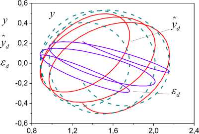
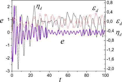
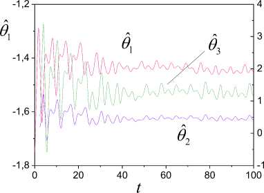
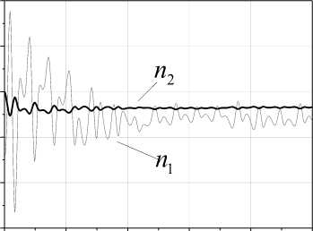
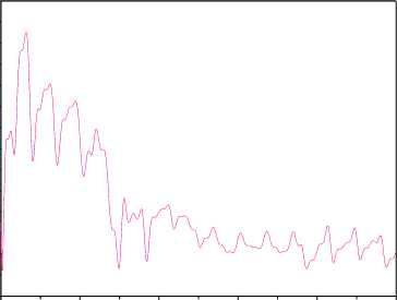
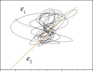
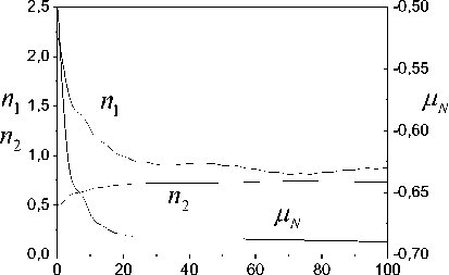
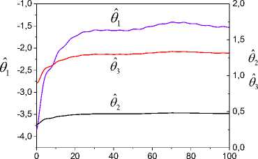
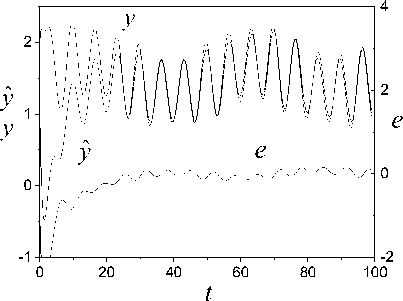
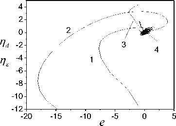
(iv) such functions sp (t) > 0 exist that vp(t)tо)&(Vp(tо)

• (v)    the upper solution of the system (39) satisfies to the vector system of comparison

^Se,Mn (t) = ^AMN^Se,Mn (t) + ^FMn ,

Where Se, Mn =[ sesMN jT ;

• (vi)    uncertainty h (t) = o^ (t)P(t) in (31) is restricted.

Then ASEN -system is exponentially-dissipative and estimations are fair

t

V(t) < eA^{MN (}t^-t⁰)S_e,m (10) + J e^A™⁽t-^T)Fm_n(t) dT , t₀

V (t) < a max I i^An 11^{2 e}i, m (t) । t ^",

If

228 к > 0 , k dNYN > g dN , t where S1 (t) is the first column of the matrix J eAV(t-T) dT .

t₀

The proof of theorem 6 is given in Appendix H.

Theorem 6 shows that properties the ASEN -system depend on the quality of work the adaptive algorithm (18). Therefore, the maximum dimension chooses N(t) for the decrease of the misalignment A^ (t) . Explain it to that quality of the tuning N(t) influences on the magnitude of the error e(t) and г .

• VIII.    Results of Modeling

Consider object (1) second order with parameters av (t) = -2 + 0.3sin(0.04^t) , b = 1.5

a₂ (t) = -3 + 0.5 sin(0.09^t) ., r(t) = 2 + sin(0.3^t) .

The equation (1) was integrated with the step 0.2s. x(0) = 2, x(0) = 1. The informational set I_o is obtained for the object (1). Parameter of the auxiliary filter (5) Л = -1.5, P (0) = 0, P_r (0) = 0. к = 1.

Consider SED -system. Apply the following approach to the definition of the variable г. Fulfill segmentation of values the variable y(t) on set J on the basis of observance of a condition structural homogeneity of modification y(t). Apply the method described in section 5, and find the vector H_d on each subinterval J c J . Choose the value H ensuring the maximum of determination coefficient for model ;y_d = HTTP. We will obtain the vector H_d =[0.28; - 1.19;0.59]T on the interval

[39.2; 79.2] s. Fulfill the prediction of change y(t) by means of the model y_a = HTTP and determine ^. Next, use the obtained variable ^ for implementation SED -system. Show change e_d in Fig. 1.

Fig.3. Change error e , ^ and the uncertainty estimation n .

y

Fig.1. Uncertainty estimation in object (1) on the basis of application SED -system.

Determine the matrix H for implementation SED -systems. Apply the approach described in section 5. The vector H = [-1.75;0.65;1.8]T in (6) is obtained on the time gap [12.2; 19.2]s. The matrix H is obtained on the basis H

Changes of the error e(t), ^ , and the calculated current value n = ^A uncertainty are shown in the Fig. 3.

Show in the Fig. 4 change of parameters 6 (t) 6₂ (t) 6₃ (t) J = HN(t). Tuning of the variable ^ in system (26) is presented in Fig. 5. Parameters of object (1) after reduction of its equation to the form (4) varied in ranges:

6 (t) = [-1.95;-1.25], 6 (t) = [0.4;0.95], 6 = 1.5.

-1.75

0.65

1.8

The vector N(t) e R² is tuned by means of algorithm (18). Matrix Г in (18) has the form Г = diag (0.005; 0.05). Factor y_g in (26) y_e = 5 . Results of work SED -system are shown in Fig. 2-6.

The Fig. 2 represents the process of tuning of the vector N(t).

^

Fig.4. Parameter estimations of the object (4), obtained by means of system (26).

2,0

n1 1,5

n2 1,0

0,5

0,0

-0,5

0       20      40      60      80      100

t

Fig.2. Tuning of the vector N(t) by means of the algorithm (18).

4 v_s

-2

-4

0       20      40      60      80      100

t

Fig.5. Change of the parameter ^ the system (26).

The analysis of obtained results confirms workability the adaptive SED -systems. Explain such change: (i) application of a static model (SM) for uncertainty identification; (ii) obtaining of parameters SM on the given time gap. This note is true for change of elements of the vector N(t). Work of the adaptive observer is stabilized at the increase of parameters tuning time.

We give the comparison of results work SED -system with one and two adjusted parameters (Fig. 6). Designate relative values of errors SED -systems with N∈Rand N∈R² as e(t) and e(t). Except the initial stage of tuning of the vector N(t) the model (26). The Fig. 6 shows of the framework change described by the function f (e ) : e (t) → e (t) . S shows the comparative position e(t) and e(t), starting t ≥ 19.2 s. We see that an accuracy of the adaptive system with N∈R is lower, than with N∈R² . The framework S is more informative than change e on t the plane (t, e) . We have made this conclusion on the basis of the theorem 6 for the ASEN -system. It is also true and for ASED -

NµN                                             Nµε system.

0,6

0,4

^e1 0,2

e₂0,0

-0,2

-0,4

-0,6

-0,75 -0,50 -0,25 0,00  0,25  0,50  0,75

e₂

Fig.6. Comparison of the work quality of the system (26) with one and two adjusted parameters

Consider the work of ASEN -system. The matrix Nµ_N

H has the form (40), N(t)∈R² . Matrix Γ in (18): γ=diag(0.004;0.0007) . The factor γ_N SEN -system is 0.0006. Show results of the work ASED -system in Nµ_N

Fig. 7 - 10. The Fig. 7 represents tuning of the vector N(t) the system (28).

Compare these results with the parameters tuning of the system (26). We see that adaptation process in the ASEN -system has monotonic character. Explain this the adequate estimation of the uncertainty h(t).

Present in the Fig. 8 identification results of the object (4), obtained by means of the system (28). The Fig. 9 contains results of the work ASED -system. We see NµN that the adaptive system is exponentially-dissipative.

t

Fig.7. Tuning of model parameters, the system (28).

t

Fig.8. Estimations of parameters the object (4) obtained by means of the system (28).

Fig.9. Estimation of adequacy work system (28)

Fig.10. Identification results of the uncertainty by means of systems (26), (28)

Loop estimation work results of the uncertainty object at different parameters of systems (26), (28) are presented in the Fig. 10. The designations applied in Fig. 10: 1 is systems (26) with N(t) g R and the static law n = 0.9^ of the estimation h^ (t); 2 is systems (28) with N(t) g R2 and the static law n = ^ ; 3 is systems (28) with N(t) g R2 and the algorithm A = -yNesN ; 4 is systems (26) with N(t) g R and the algorithm A = -y£ eed . Results are presented in the form of the frameworks described by functions f : e(t) ^ n (t) , i = d, N .

The analysis of the Fig. 10 shows that best performances have the adaptive SEN -system. Remaining variants of the considered systems have the large time tuning and a low accuracy of the uncertainty estimation.

• IX.    Conclusion

The method of construction adaptive observers for time-varying linear dynamic objects is proposed at nonfulfillment of the condition excitation constancy. The problem of synthesis AO is divided into two subtasks. The first problem proposes the procedure to the choice of the constant matrix, allowing decreasing effect the excitation constancy condition. This matrix superimposes restrictions on parameters AO. The solution of the second task gives to the choice of adaptive algorithms on the basis of the obtained matrix. We introduce the set of multiplicative adaptive parameters, allowing identification problem under restrictions to solve. Adaptive algorithms of multiplicative identification are designed.

Two methods of an estimation uncertainty are proposed for improvement performance of the adaptive observer. The first method is based on a design of a static model for the uncertainty estimation. We introduce the parameter improving the accuracy of the uncertainty estimation. The second method gives the uncertainty estimation on the basis of parameter current values the adaptive observer. The exponential dissipativity of the adaptive observer is proved. We present the results of the modeling confirming effectiveness of designed methods and procedures.

Appendix A. Proof of Theorem 1

Consider Lyapunov function V(t) (30). The choice of the second component in the right part (30) is substantiated in [15]. Find the derivative V(t) on motions AS^ss -system. Obtain after simple transformations for V(t) the inequality

V <-2Ve - ys^V, (A.1)

where q = minpJTP .

Apply the condition 1) of theorem 1. Then we obtain from (A.1), what V(t) < 0 and the system ASs_n is stable. Integrate (A.1) on the time and obtain

t

V(to) -J(2V(t) + yq42 V(t) )dT > V(t).

t₀

As V (e,^, a) satisfies the condition 1) theorem 1 then all trajectories of the system AS^ss belong the area Gt ={(e, N, a) : V(t) < V (t0)} . Then we have the estimation for AS^ss -system

t

J(2Ve(t) + rq42Ve(t))dT< V(to) -V(t).

t₀

Obtain the inequality (29). Consider V(t)

Ve =^-ke^{2 +}eSNP^-Ys |e||H<

(A.2)

Use the inequality [21]

- az¹ + bz< —az— + —,  a > 0, b > 0, z > 0

22a and transform (A.2) to the form

Ve <-k!^e ’ + Tk^(l^'^|И + Y.lz )2.      

Present (A.3) after simple transformations as

V_e<-kV_e +¹1 UP max k V t

(A.4)

where o_p = max|p(t)||2, u_z = max|z(t)|.

From (A.4) we obtain the estimation (29) for V(t).

Appendix B. Proof of Theorem 2

Consider Lyapunov function

t

V(t) = Ve(t) + J^T (t)Г 'TN (N)3N(t)dT t0

.

t

+J ^vT^rtsT a (Ц)Ц(т ) dT t0

Transform V(t) on motions of the system AS^ds to the form

V<-2Ve .

(B.1)

V satisfies to the condition 1) theorem 1. Obtain from

• (B.1)    the inequality V(t) < 0 . AS^ds -system is stable. Integrate (B.1)

∫^t2Ve(τ)dτ≤V(t0)-V(t) .           (B.2)

t₀

Obtain from (B.2) the boundedness of trajectories AS_N^ds_µ -system.

The estimation for V has the form

Ve≤-^k₂e²+₂¹_k(δNIlli^PII ⁺I^zI)².

Obtain from (A.2) the estimation (29) with γ²= 1 .

• Appendix C. Proof of Theorem 3

Consider Lyapunov function

• Veµ(t)=Ve(t)+γd^-1∫^tµ(τ)Ψµ(µ)µ(τ)dτ=Ve(t)+Vµ(t). t₀

Present V as eµ

V_e+V_µ=-ke²+eδ_N^TP≤-^ke²+υ^P max δ_N(t)II².

Then

V_e(t)≤υ^P₂ max δ_N(t) ²-∫V_µ(τ)dτ. t₀

Let Ψ(µ) =1 . Then have

• V_µ(τ)dτ= ¹(µ²(t)-µ²(t₀))>0 .

_t0             2γd

So

V_e(t)≤υ^P₂ max δ_N(t) ².

• Appendix D.    Proof of Lemma 1

Consider V(t)

VN(t)=-eΔ^TNPH .            (D.1)

To ensure property V(t)∈M apply the approach [15, 18]. Let for (∀t ≥ t^*> t )&(∀(e,Δ )) ∈O (O)) the condition is satisfied

O ={0, 0m}⊂R×Rm×J0,∞, where O = {0, 0l} ⊂ R×Rl×J is the equilibrium position of the system, Oν (O) is some neighborhood of the point O , 0l∈ Rl is the zero vector, t∈ [0, ∞] = J, ϑ> 0 is some number.

Transform (D.1) to the form [15]

VN(t)=-ϑ(Δ^TNBHΔN +e²) .

Next use (32) and the approach described in [18]. Let Ψ (N)=P(N)=I . Then obtain

• VN ≤-³aϑΔ^TNΔN +

.

²ϑe²≤-^3αϑλ1(Γ)V +⁴ϑV⇔V∈M⁺

3              4      ^N3^eδ

• Appendix E.    Proof of Lemma 2

Apply (31) and present V as

• V    ≤ -ke²+ I^eI δ_N^TP_H +σ_Δ^TP+µz I .        (E.1)

We obtain from (E.1) V∈M . Ensure the condition

• V∈M⁺. Apply the proof of the theorem 1 and obtain

V_e ≤-^ke²+ ¹(Δ^T_NP_H +σ_Δ^TP+µz)²≤

• -kV + (2αλ(Γ)V +υ maxIσ_Δ(t)II²+υ_z ). k^t

So, property V∈M⁺for V has the form

V_e ≤-kV_e+²αλ^l(Γ)V_N + ¹ (υ_P maxIσ_Δ(t)II²+υ_z ).

Appendix F. Proof of Theorem 5

Consider Lyapunov function

V(t)=Ve(t)+0.5γε^-1µ²(t)=Ve(t)+Vµ(t).

Write V as

Apply the proof scheme of theorems 1, 2 and obtain

V<-kVe +1 [amax]|Д.(t)||2 + ®] ,       (F.1)

where maxh2(t) < to, to — 0 is some number. The inequality (38) follows from (F.1).

Appendix H. Proof of Theorem 6

Show boundedness of system ASED trajectories. Let such number p _лexists that the equality hд (t) = p*,.sN (t) is true.

Consider Lyapunov function

V (t) = Ve (t) + V^N (t) + V. (t) =

0.5e2(t) + 0.5yN (Sp.(t))2 + 0.5^2 (t |Г V (t), where Sp. = PN - p* ..

Write V as

^V ke + e^Д_N^PH⁺eS/djNSN  eSpN^N  e^Дn^Ph . (H.1)

Therefore, we have V< -2kV_e. Integrate this inequality and obtain

• V (t) < V(10) - 2kjVe(t)dT .          (H.2)

t₀

Hence, all trajectories of the system ASED belong area Q = {(e, Д.,SpN): V(t) < V(1₀)} .

Consider Lyapunov functions V(t)    and

V_pn (t) = 0.5 (dp_N(t))2. Transform V to the form

Ve = - ke² + e Д ^T_NP_H + eSpN^N.       (H.3)

The vector P has property PE . Apply the proof scheme of lemma 1 and ensure for V_e property V_e e M⁺ in the form

Ve = -ke2+eДNPH + eSPNsN <

• ^- ke² + |e| |^ДNPH + Зд,^| <

• -    ke²+1 [||Д ,| П IP,11¹ * )²s. ]<    <^H.4)

• -    ^kVe^{+ a} max 1^ДN I^{1 +}^VN ■

where s2 < d_N, d_N — 0 is some number.

Ensure the condition V^ e M⁺. By analogy with (H.4) obtain

• V Pn = -YNeSPNSN = -U(/NSPNSN + e2 ) =

• f    1             ^ 2

• - UI e + - YNeSPNSN I + UYNeSpNgN

• - oyNspN,sN + UyNspNsN <          (H.5)

• <    — °YnSPn sN + uYn \e5tNSNM | <

• ^- -^udNYNVPN^{+ uV}e.

As и does not influence on properties of the system assume и = 1 . So, we have for V_e and V^ following inequalities

Ve

V pN

- k и

2dN k дUdNYN

V

^PN ]

(H.6)

a max ||^Дn|I²

Let S = ^[s s 1 , ^e, ^pN    L ^{e P}N ]

A =	-k	2dN k	, F =	a max 1д.1
Pn		3	’   PN
	u	-- UdNYN		_       0       ]

Let such functions s_p (t) > 0 exist that

• ^VP(t) <Sp⁽t) V(t > t0)&(Vp (t0)<sp (t0)) , p = ^e, Pn .

We obtain the vector system of comparison for (H.6)

^Se,Pn (t) = ApNSe,д. (t) + FpN -         (H.7)

Stability conditions of the system (H.7) have the form

228 k > ⁰ , k dN^Y. —  ^dN .

Hence

t

• V(t) < eA^PN(t^-t⁰)Se,PN (10) + JeA^PN(t^-T)Fpn (t)dT .

t₀

Limiting properties the ASED -system estimate as

V(t) ≤ k mtax IIΔN2Σ1,µ(t)t→∞, where Σ (t) is the first column of the matrix t ∫eAV(t-τ)dτ.

t₀