Adaptive Observers with Uncertainty in Loop Tuning for Linear Time-Varying Dynamical Systems

Author: Nikolay Karabutov
Journal: International Journal of Intelligent Systems and Applications(IJISA) @ijisa
Article in issue: 4 vol.9, 2017.
Free access
The method of construction adaptive observers for linear time-varying dynamical systems with one input and an output is offered. Adaptive algorithms for identification are designed. Adaptive algorithms not realized as an adaptive system contains parametric uncertainty (PU). Realized adaptive algorithms of identification parameters system are offered. They on the procedure of the estimation PU and algorithm of signal adaptation are based. The algorithm of velocity change system parameters estimation is proposed. Estimations PU and its misalignments are obtained. Boundedness of trajectories an adaptive system is proved. Exponential stability conditions of the adaptive system are obtained. Iterative procedure of construction a parametric restrictions area is proposed. Simulation results have confirmed the efficiency of the method construction an adaptive observer.
Identification, adaptive observer, time-varying dynamical system, Lyapunov function, uncertainty, vector combined equations of comparison
Short address: https://sciup.org/15010916
IDR: 15010916
Text of the scientific article Adaptive Observers with Uncertainty in Loop Tuning for Linear Time-Varying Dynamical Systems
Published Online April 2017 in MECS DOI: 10.5815/ijisa.2017.04.01
Construction of adaptive observers (AO) is one of the rapidly developing areas of control theory. The basis of theory AO for the linear class of dynamic systems has been obtained in the end of past century [1-6]. The class of the adaptive systems having special identification representation in space "input-exit" has been proposed. Despite this, the research in this area continues. In particular, attempts of construction AO for time-varying plants are made. The majority of the approaches are based on the generalization of the results which are obtained for linear time-invariant dynamic systems.
Problem of combined identification and control of the discrete dynamic system with time-varying parameters is considered in [7]. It is supposed that parameters are piecewise constant, and the modification time is determined by means of the Markov chain. Convergence of adaptive algorithms is proved. The set of criteria allowing minimizing an error of forecasting an output system, is applied to improve efficiency of control. Such approach complicates identification systems. Problem of adaptive identification time-varying nonlinear plant is considered in [8]. It is supposed that the plant state vector is meas- ured and description of a nonlinear part of the system is known. The unknown vector of parameters system approximates Taylor series. The adaptive algorithm of identification is offered. Lüders-Narendra adaptive observer [9] is applied to stabilization of time-varying nonlinear continuous system. Boundedness of trajectories in an adaptive system is proved.
Methods of adaptive control dynamic systems with variable parameters are proposed in [10]. It is supposed that parameters have the restricted velocity of a change. Boundedness of trajectories in an adaptive system is proved. This approach improves the quality of transients in an adaptive system. It on nonlinear time-varying systems can be generalized.
A multidimensional linear time-varying dynamical system is considered in [11]. Matrix state and control has the known function of time. It is supposed that the linear part of the system depends on an unknown parameter vector. The adaptive Kalman filter for a state estimation and system parameters is offered.
Considered methods and algorithms do not allow to ensure the unbiasedness of obtained estimations [12, 13]. Explain it to that the law of a change parameters is unknown. Therefore, the majority of approaches on a quasi-stationary hypothesis are based.
The solution of the adaptive identification problem time-varying systems is based on application: i) various methods of parameters approximation [8]; ii) compensating controls [9, 14]. Choice of the reference model in [14] is realized on the basis of the prior information analysis. The law of parameters modification under the priori uncertainty is unknown. Therefore, the object as a system with parametric uncertainty is considered.
AO application for control of the stationary uncertain object is given in [3, 15]. The case when uncertainty is a discrepancy of model to plant (structural disturbances) is studied. Such disturbances are called non-modeling dynamics. Algorithms which ensure robustness to these disturbances are designed.
Integrated algorithms of the identification parameters vector of time-varying linear system are designed in [16]. The law of change unknown parameter drift system is specified as a dynamic system with unknown constant parameter vector. It is specified in the process of adaptation. Dynamic system with a time-varying matrix of a state is considered in [17]. The matrix is specified a priori.
The problem is reduced to identification of unknown constant parameter vector. The adaptive algorithm of tuning is proposed.
So, the problem of identification time-varying systems as before is actual. The problem of ensuring the asymptotic stability of the adaptive system in the output space is not solved. The problem of system identifiability at nonperformance of excitation constancy data condition was not studied.
We for linear time-varying dynamical systems propose a method of construction AO with uncertainty in a loop tuning. Algorithms of tuning parameters AO are developed. The dynamic system for estimation the velocity of system parameters change is proposed. The system parameters are formed in the synthesis process of the estimation system. The algorithm of signal adaptation for compensation of non-modeling dynamics is developed. Boundedness of trajectories adaptive system with AO is proved. Conditions of an exponential stability adaptive system are obtained.
The paper has the following structure. Section 2 contains the problem statement. The design of adaptive algorithms is described in section 3. The Lyapunov functions method is applied to obtaining of adaptive algorithms. Obtained adaptive algorithms are unrealizable. Therefore, we propose dynamic system for change velocity estimation of initial system parameters. It is showed that this system has linear form and depends on an unknown constant vector of parameters. The design of an algorithm for estimation of the unknown constant vector of parameters is given in section 4. Choice of dynamic system parameters for estimation of change parameters velocity of initial system is given in section 5. Properties of the developed adaptive identification system are researched in section 6. The definition method of the guaranteed parameter estimation area AO is described in section 7. It is based on processing of experimental data set in "the vertical direction" (on range), and represents the intellectual procedure of decision-making. Simulation results of the obtained AO are presented in section 8. The final section contains the review of obtained results and their discussion.
-
II. Problem Statement
Consider dynamic system
X = A( t ) x + b ( t ) r , y = C T X ,
where X e Rm is a state vector, r e R , y e R is input and output of system, A e Rmxm is matrix of state the form ed, but a priori unknown area G ,; ЛеR(m-1)x(m-1) is stable diagonal matrix; B e Gs c Rm , GB is restricted, a priori an unknown area; H e Rm-1, h = 1 (i = 1, m -1) , C e Rm , C = [ 10 K 0 ]T . The pair (Л, H) is controllable.
Assumptions.
A1. The input r ( t ) is a piecewise continuous bounded.
A2. || A ( t )|| < a , || B (t )|| < в , a > 0, в > 0.
A3. The transitive matrix of the system (1) is uniformly restricted on a time.
Apply model to identification of pair { A ( t ), B ( t ) }
5c = am (5c - cctx )+A (t) y+B (t) r, y = CTX, where AM e Rmxm is the Hurwitz matrix of the form
AM =
- k

k > 0; vA e Rm , BB e Rm are vectors of adjusted parameters; 5B e Rm is state vector; y e R is model output.
For system (1) we have the information
I o = { y(t ), r ( t )> t e J } .
Problem: construct the model (2) and determine such laws of tuning of vectors Aˆ (t) and Bˆ (t) on the basis of the analysis I for the system (1) satisfying to assumptions of A1-A3 that lim| y (t)- y(t)l < Sy,, Sy > 0 . t ^да y y
-
III. Synthesis of Adaptive Algorithms
Write the equation for the prediction errors. Subtract (1) of (2) and obtain
E = AME + SAy + SBr, e = CTE, where SA(t) = Jf(t) - A(t), SB(t) = BB(t) - B(t) are vectors of parametric misalignments.
Apply to y ( t ) and r ( t ) auxiliary filters
P v =Л P v + Hv , v = y , r , (4)
A e G^ c Rm is vector of parameters, belonging restrict
where P e R m - 1 , P e R m - 1.
Let 3 D(t ) = [ 3 A T (t ) 3 B T (t )] T is the vector of misalignments parameters system (1), 3 D e R 2 m , P e R 2 m is the vector of the generalized input, P T = [ y P T r P T ].
Lemma 1.
e = - ke + 3DTP -A^,(5)
where A ^ e R ,
A ^ = A ^ ( 3 D , P , t ) , 3 D 2 = 3 D \ { 3 a ,, 3 3 ,} .
Proof. Obtain for e(t) the equation e = CTE = -ke + 3axy + 33 r + Ht E^,(6)
where ET = [ e E T ] ,
3 AT = [ 3 a, 3 A TT ] , 3 BT = [ 3 31 3 B2T ] ,
E2 =( sIm-i —Л)-1 (3A y + 3B2 r),(7)
s = d / dt , Im_ , e R ( m - 1) x ( m - 1) is unity matrix.
Considering (4) and (7), HTE transform to the form
HE = 3 A TP + 3BTP - A^ ,(8)
where t
A ^ ( t ) = J [ 3 A2t ( t - t ) 3 B T ( t - t ) ] [ P T ( t ) P T ( t ) ] d T . t 0
Substitute (8) in (7) and obtain (5).
We see from the equation (5) that the error e ( t ) depends as on the unknown vector 3 D ( t ) , and a velocity of its change (function A ^ ( t ) ). 3 D ( t ) £ Ia ( Ia is an a priori information). Therefore, consider A ^ ( t ) as uncertainty of the system (5). A ^ ( t ) does not reflect the effect of the change velocity parameters a ( t ), b ( t ).
Integral algorithms of identification the vector D ( t ) are designed in [16]. Here we are offered the new approach to estimation of the uncertainty A ^ ( A D 2, P , t ) in system (3). We show, as on the basis of estimations A ^ ( t ) to determine the parameter vector D ( t ) ( D ( t ) called drift parameters).
Apply Lyapunov function Ve = 0,5 ET (t)CCT E(t ) for algorithms design for tuning of parameters the model (2). Derivative V on the time note as
V = -ke2 + e3DTP - eA^.(9)
Obtain [18] from the condition Ve < 0
3D (t) = -Fe (t) P (t),(10)
D (t) = D (t)-Fe (t) P (t),(11)
where Г = Г T > 0, Fe R 2 m x 2 m is a matrix ensuring convergence of algorithm.
The vector D ( t ) in (11) specifies the dynamic law of the change parameters system (1) and it is a priori unknown. Therefore, the law (11) is not realized. We will estimate the vector D in the identification process. Write algorithms (10), (11) in the form
D (t ) = Z (t ) -F e ( t ) P (t ), (12)
3 D(t ) = 3 2^ ( t ) - F e ( t ) P(t ), (13)
where i Z e R2m is an estimation of the velocity change parameter vector D ( t ), Z(t ) = D ( t ) .
Name algorithm (12) realized. Adaptive identification algorithms of time-varying systems in such form are considered for the first time. Most often, the vector D ( t ) is estimated on the basis of Kalman filter [12]. We estimate the drift of parameters as a state of some dynamic system.
Present the vector Z ( t )as [18]
Z(t ) = - LD(t ) + Q(t ) K , (14)
where L e R 2 m x 2 m is diagonal matrix with lu > 0 ( i = 1, 2 m ) , Q e R2m x n is matrix with known elements, K e Rn is an unknown vector with constant elements.
The matrix Q ( t ) we form a priori. It sets drift of the change of the vector D ( t ), i.e. qy e Q с Ф , where O ( t ) = { ^ . ( t )} is the set of given functions.
So, the law of the change vector D ( t ) the system (1) is specified on set Ф . Change D ( t ) depends on an unknown vector K .
Write adaptive identification algorithms (12), (13) as
f)(t ) = - LP)(t ) + Q ( t ) KK ( t ) -F e ( t ) P ( t ), (15)
3 D(t ) = - L 3 D(t ) + Q(t) 3 K(t ) - F e ( t ) P ( t ) . (16)
We have reduced the identification problem to the definition of the law the estimation vector K .
The criterion V ( t ) to synthesize identification algorithm of the vector K does not allow. In the next section, we proposed a method of estimation the vector K .
-
IV. Algorithm of Estimation Vector K
We propose a method of the estimation vector K . It is based on implementation of two stages. At first, we estimate the unobservable variable AoU ) = Ao ( 5 D, t ) . Next, use estimation A o ( t ) for the tuning of vector K . The algorithm design for the tuning K ˆ is based on introduction of an auxiliary error. The auxiliary error is the basis for variable estimation A o ( t ).
Describe the method of estimation the unobservable variable A o ( t ) = A o ( A D , t ) . Form criterion of algorithm tuning synthesis of the vector K ˆ in (15) on the basis A o ( t ).
Apply to the vector P ( t ) the auxiliary filter
Pk = -kPk + P.(17)
Lemma 2.
y = kpY_k + DTP - оk,(18)
e = 5DTPk -Atok,(19)
where px k e P is the first element of the vector P ,
t оk (t) =J DT (t -t)Pk (t)dT .(20)
t 0
Proof. Consider the first equation of system (2)
-
y = - ke + a y + bx r + H T XX2 .
Transform it to the form y = - ke + ax y + b r + W., (5 )T (ATy +13Tr), (21)
where W ( s ) = ( sIm_ T - Л ) - 1 H is transfer function, X = [ y X) T ] T .
Divide the left and right parts (21) on s + k , s = d/dt. Apply (17) and obtain y = kP1,k + DTP - оt,(22)
y = kP1, k + yk,(23)
Where yk = IT [a y + b r, XXT]T / (s + k), I =[1 HT]T,(24)
-
O)k (t) =JDT (t -T)Pk (t)dT .(25)
t 0
Subtracting from (20), we obtain (19).
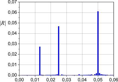
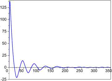
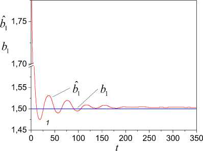
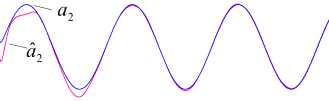
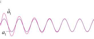
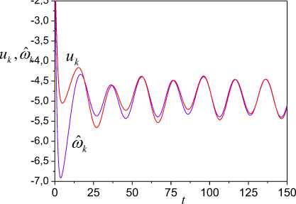
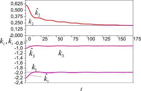
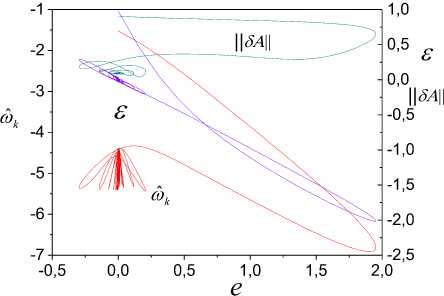
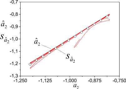
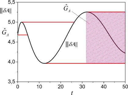
The proof of lemma 2 (see (23)) and (18) gives the following estimates y = kP1, k + yk, yt = I)TP - y^ (t) is known for any t > t0. Therefore, obtain uncertainty estimation from (26) 6>k (t) = D)T (t)Pk (t)-yk (t) Vt > 10.(27) Apply the following approach for obtaining о (t) . Designate uk (t) = о (t) and (18) write in the form y = kP1,1 k + DTPk - Uk,(28) where uke R is the compensating control. As at the identification stage uk (t) ^ о (t) almost Vt > t0, we use in (28) the designation y(t) instead of yˆ (t). Subtract y(t) from (28) and obtain the equation for auxiliary error e(t) e(t) = 5D (t)Pk (t) - uk (t) + Ok (t), (29) where e = y - y. Define u(t) from the condition Uk = arg min Vu, uk and obtain uk = Yke, where V (t) = 0,5e2 (t), yk > 0. Then the estimation for A^ (t) is fair: £(t) = <уk (t)- Uk (t). ^(t) is described with the differential equation к = (-LAD + Q5K - reP)T P .(32) Consider Lyapunov function V (t) = 0,5к2 (t) . Determine adaptation algorithm of the vector Kˆ in (15). Ap ply (32) and write V(t) as Ve = -ePLSD + ePQSK - eePTk ГP. (33) Then SK = K = -fk^QPk, (34) where f e R"x", f =fT > 0. So, the adaptive identification system is described with equations (3), (4), (16), (27), (30) - (32), (34). Remark 1. Approaches based on use of the expanded error [19], do not allow to form criterion for the estimation function Am (t) . Therefore, we have applied indirect methods to the estimation of uncertainty. We define estimation e(t) uncertainty A^ (t) on the basis of the current values of the model parameters Dˆ (t) and apply the algorithm (34). V. About Choice of Matrix Q(t) in Algorithm (16) The equation (14) describes dynamics of change vector D(t) and has the general form. Its properties depend on the choice of matrixes Q, L and the vector K . As a rule, the structure of the adaptation law (matrix Q,L,K) is set a priori. Matrix elements Q(t) can be set posteriori on the basis of the preliminary analysis the set I . Let the frequent spectrum of signals y(t), r(t) is known, i.e. is the set Q = {Q, Qr}. As the linear dynamic system (1) is consider, frequency set for the vector D(t) define as QD =Q, \Qr. Specify O(Qn) on the basis QD and generate the matrix Q(t). VI. Properties of Adaptive Identification System We will consider properties of the proposed AO. The system is complex and has several levels. We will apply Lyapunov vector functions method to the proof of the adaptive system stability. Consider the condition of extreme nondegenerate (the constancy of excitation) vector P(t) [20]. Lemma 3. The estimation for an informational matrix P(t)PT (t) is fair ""D(t)< ||P(t)PT(t)||< <(t) Vt > 0, (35) where P(t) e R2m is the generalized input of system (5); "< 2m is the rank of matrix P(t)PT (t) ; Dn (t) is the largest nonzero principal minor of the matrix P(t)PT (t) ; ^P (t) is maximum eigenvalue of the matrix P(t)PT (t); P(t)PT(t) is a norm of the matrix P(t)PT (t) . Theorem 1. Let are fulfilled assumptions А1-А3 and conditions: 1) all trajectories of system (1), (2) uniformly are bounded on t ; 2) positive definite function V(e, e, AA, Л, t) satisfies condition inf V(e, e, 3D, SK, t) ^ ^ if 11 [e e SDT SKT ] || ^ ”; 3) the matrix Q(t) in (34) and vectors P(t), P(t) are extreme no degenerate and satisfy (35); 4) the matrix Ler2mx2m in (14) is the diagonal with ltt > 0 ; 5) e(t)e(t) > ae2(t), a > 0 . Then all trajectories of system (3), (4), (14), (16), (27), (30) - (32), (34) are restricted. Lemma 4. f Qf-1 SD = ef kQPk.(36) Proof. Consider function VS(t) = 0,53DT(t)f-1 SD(t) .(37) V(t) has the form V =-SDTf-1 LSD + SDf-1QSK-eSDTP.(38) Obtain from the condition V5 (t) < 0 adaptation algorithm for the vector SK(t) SK = -f k QT f-1SD,(39) where f eR"x", f =fT >0. Compare (39) and (19) and obtain assertion of lemma 4. Lemma 5. A^ (t) = cSe( t), where S > 0, 0 < c < 1. Proof. A^(t) write as A^(t) = ce(t) , where 0 < c(t) < 1, A®(t) = j SDT (t - r)P(t)dT . (40) t0 Present P(t) as function from P(t). Obtain from (17) at Pk(t0)=0 Pk(t)=∫texp(-kI2m(t-τ))P(τ)dτ. t0 If the integration step ∆t is small enough and assumption А1 is fulfilled, then Pk(t) =ϑ-1P(t), where ϑ= k/(1 - exp(-k∆t)) . Determine P(t) from last equation and substitute it in (40). Consider equality (31) and obtain assertion of the lemma 5. Proof of Theorem 1. Consider Lyapunov function V(e,ε,δD,δK,t)=V (e,t)+V (ε, t) + Vδ(δD,t)+VK(δK,t), Where VK(δK,t)=0,5δKT(t)(Γk-1+Γk-1)δKT(t), Ve(e,t)=0,5e2(t), Vε(e,t)=0,5ε2(t), V (δD,t) have the form (37). The time derivatives of the function components V(t) described by the equations (9), (33), (38) and VK =-δKT(In+Γk-1Γk-1)εQTPk .(41) Sum (9) and (38), (33) and (41): V =V +V =-ke2-e∆ω -δDTΓ-1LδD eδ e∆ 2 ,(42) +δDTΓ-1QδK VεK =Vε+VK =-εPkTLδD-εePkTΓP -εδKTΓk-1Γk-1QTPk Determine δD from (36) and substitute it in (42). Apply the lemma 4 to last summand in (43). Then VεK =-εPkTLLεPk -εePkTΓP-δDTΓ-1QδK,(44) where Lε =Γ(QQT)-1QΓk-1ΓkQT. The matrix Q(t) and vectors P(t), P(t) satisfy conditions 3) theorem 1, and matrix L satisfies to a condition 4) theorem 1. Matrixes Γ , Γ and Γ are symmetrical positive defined. Therefore, following inequalities are fair PkTLLεPk≥µε, PkTΓP≥µ, (45) where µ=ΓIImin min Pk(t) minIIP(t)II , µε= LminLεIImin t IIPk(t)II , || ⋅ || is lower boundary of norm matrixes L and L . Obtain from a condition of passivity of the adaptive system eε ≥ 0 , eε≥ αεe2 , 0 ≤ αε .(46) Apply (45), (46) and (44) write as Vεk ≤-µεε2-αεηe2-δDTΓ-1QδK .(47) Sum (42), (47) V =-ke2 -e∆ω -δDTΓ-1LδD- µε2 -αηe2 .(48) Apply lemma 5 to ∆ω . Then obtain for e∆ω the estimation e∆ω2 ≥ сωe2 ,(49) where с =ϑα c , c = minc(t) . Let λmin(L)≤L ≤λmax(L) , where λmin(L) >0 , λ (L) > 0 are minimum and maximum eigenvalues of matrix L . Then δDTΓ-1LδD≥2λmin(L)Vδ.(50) Apply (49), (50) and for V obtain the estimation V ≤-2(kVe+λmin(L)Vδ+µεV) ,(51) where k= k+αεη+сω>0 . V is negatively definite on variables e,ε,δD. Therefore, the estimation is fair V(t)≤V(t0)-σ(t),(52) σ(t)=∫t2(kVe(τ)+λmin(L)Vδ(τ)+µεVε(τ))dτ. t0 Functions V (t), V (t), V (t) satisfy to the condition 2) theorem 1, and function V(t) is positive definite ∀t≥t. Hence, we obtain from (52) boundedness of all trajectories in еhe identification system. Definition 1 [20]. The non-positive quadratic form W(Y, X) has M -property or W(Y, X) g M, if it is representable as W (Y, X) = - cJY |2 + c^, (Y, X), for any Y g Rm, X g Rn in limited area nD ={y g Rm, X g R"| YI2 +|X I2< a, a > 0 }, where ||Y|| is Euclidean norm of a vector Y , c > 0 , c^ > 0, W^ (Y, X) is some function. Definition 2 [20]. The non-positive quadratic form W(Y, X) has M+-property or W(Y, X) g M+, if it is representable as W (Y, X) = - CyYII2 + Cx||X||2, for any Y g Rm , X g Rn in restricted area Qn , where cx > 0. M+-property is an indication of constructive completeness the quadratic form W(Y,X) . It allows analysis of properties W(Y, X) to reduce to the estimation of indexes corresponding M -matrix. Estimate asymptotic stability of the designed adaptive system. Consider Lyapunov vector function V(t) = [V (t) V (t) V6(t) Vk (t)]T, where V. (t) = 0,55KT (t)Г-15K(t). Set positive functions s, (t) for V (t) Vt > t0. st (t) is majorant for V (t), where s (t0) > V (t0), i = e, 5,e,k . Lemma 6. Vector equations system of comparison for V(t) Proof. We have for the derivative V(t) the equation (9). Write the equations for derivative other elements of the vector V(t) V = -5DT Г-1 L5D + 5DT Г-1 Q5K - e5DT P,(55) V = -ePTL5D + ePTQ5K - цве,(56) Vk =s5KTQPk,(57) where ц = PT Гp . We obtain from (9), (55) - (57) obtain that Veg M, V ^ M and VK £ M . We will ensure execution M -properties for functions V and V , and then we will satisfy the condition V(t) g M+. Consider at first (56). Apply the lemma 4 and obtain 5D = eFPk, where F = r(QQT )# Qr-1ГkQ , (QQT )# is pseudo inverse matrix. Then ePTL5D = e2PTLFP .(58) As + цс2 + це2,(59) that applies (58), (59) and (56) present in the form V = -e2PTLFP + ePTQ5K + ^e2 + це2,(60) i .e. V g M . df dfdf Let ц = max ц(t) , ц = min PT LFPk , k£ = ц - ц . Apply the inequality [21] - az2 + bz <—az— + —, a > 0, b > 0, z > 0(61) 22a where S = [se s5 se sK ]T , sv (t) > 0 , v = (e, 5, e, K) , ke > 0 , k5 > 0 , k > 0 , кк > 0 , kek5 > 2ke5 , U > 0 , 3kA (kek5 - 2k.) > 4(k.kL + k.kJk - 2kA), is exponential stable with the estimation to first two summands in a right part (60) and obtain k^e2 ( 5KTQPkPkQ5K ц^у 2 2k 2 e S(t) = eA(t-t0)s(10) , As 5KTQTPPQ3K < 2DP, that Ve<-V + EV. + kEV, (62) where kEK = Amax (ГK ) Amax (LP ) A^ (QQ ) , LP = PkPk , k = kEK k = ^ EK k£ ’ Ee 2 . So, V e M+. Go now to (57). To obtain VK e M, we 7 E V / K 7 will suppose that is true E§KTQPk = u(e2+ KKDIDOD) 3 u< 1 at t >> tQ. Apply the approach, stated in § 6.3.1 [20]. Transform V to the form V- < --u3K!Q! PPQ3K + eu3Kt QT P .(63) So, VK e M. Obtain from (63) the estimation for VK ensuring VKe M+: • , 4 VK <-kK uVK + -uV ,(64) K K K Where kK = 3 Amin (ГK ) Amin ( LP ) Amin ( QQ" ) • Now identify the estimation for V (9) ensuring property V e M+ . Apply lemma 5 and from (46) obtain eA®2 > De2 , where eto = c3a£ > 0 . Then the condition V e M+ has the form Ve<-keVe + ke5V5, (65) where ke = k + cm, k^ = Amax (LP)Amax(r) , Lp = PP is ke the matrix, satisfying conditions lemma 3. Consider (55). Ensure V5e M+. As -e3DTP = - e + -3DTP + e2+ -3DTLP3D, I 2 ) 4 that V< -3DTГ-1L3D + e2 + 3DTГ-1Q3K + - 3D Lp3D. Use inequalities 3DT Г-1L3D > A„ (Lp )3DT Г-13D, 13DLp3D< 13DГ-13DAnaX(Lp) Anax(Г) and transform (66) to the form V < -ks 3DTГ-13D + e2 + |3DTГ-1Q3K|, where ^3 = 1 (4Amin ( Lp )-An,aX( Lp ) Amax (Г) ) • Apply the inequality (61) and obtain V3<-k3 V3 + 2Ve + k3kVK, (67) where T - max max у k ) , kg 3K = k5Amm(r) , 3 = T. Use results § 6.2 [20] and obtain assertion of lemma 6. The comparison system (53) is fair for V(t). It has the solution 5(t) = eA (t-t0) S (t0). Theorem 2. Let assumptions А1-А3 and conditions 1), 3)-5) theorem 1 are fulfilled. Let: (i) exists positive definite Lyapunov vector function V(t) =[Ve (t) V3 (t) Ve (t) Vk (t)]T components which assume an infinitesimal higher limit; (ii) inequality (62), (64), (65), (67) and vector system of comparison (53), (54) are fair for elements of the vector V(t). Then the system (3), (4), (14), (16), (27), (30) - (32) is exponential stable with the estimation S (t) = eA (t- t0) S (t0), if ke > 0, k8 > 0, kE > 0, kK > 0, kek3 > 2 ke3 , u > 0, 3kKkE (kek3 -2k^) > 4(kEk3ksK + k Kk.k. -2kAK), where corresponding factors are given in the proof of lemma 6. The proof of the theorem 2 directly follows from Lemma 6. Remark 2. The lemma 6 gives the estimation of the parametric misalignment 5D(t) the vector D(t) . Remark 3. The matrix M in definition 2 for considered adaptive system has the form (54). VII. Domain of Guaranteed Estimation Section 6 contains the properties description of the adaptive identification system. We showed that the system is asymptotically stable. We propose an approach which confirms a boundedness of adaptive system trajectories in parametrical space. We will describe a method of obtaining the guaranteed parametric estimation domain G for system (1). It is based on the processing of set I in "the vertical direction" (on the range). The idea of the approach is described in [20]. We give its development on the given class of systems. Remark 4. We use the area designation G to underline its difference from areas of parametric restrictions of the system (1) for A(t), B(t) . Let on Y x U x J is specified the relation B : B c Y x U x J, J c J . Present the definition range and the range of values B as dom(B) f {J | 3(y(t) e Y)3(u(t) e U) [(Y,U) e B] } rng(B) = { (Y,U) | з(t e J)[(Y,U) e B] } . (69) Next, we consider not all range of values relation B, and its contraction By = {b |f c Yx J}: dom(By) = { J | 3(y(t) e Y) [(Y, J)e By c B] } , Cy = rng(By) = { ( YJ)| 3(J) [(Y, J) e By c B] } c R Assumption. The set С is restrictedly inf C < ^, supC < ^ , #C < ^, te J t e J where #C is cardinality of the set C . We associate the relation C with the set Iy = {y e R I y(t), t e J c J} , Iy c Io . Therefore, we will write Cy (I^ ). Remark 5. The set C can be both continuous, and discrete. Describe procedure of obtaining the estimation of the area G (I ) on set C . Let the problem of the parametric estimation on the interval Jp (t) = [t0, t] is solved and are obtained the sets E = {e e R|e (t) Vt e Jp(t)}, (70) A = {A e Rm \2(t) Vt e Jp (t)} . Consider an interval J* =[4, t]c Jp (t) where t* > t0 is the time since which the error e(t) belongs to a neighborhood O (0,^), 5e > 0. Fix any element ck e C (I^) where k corresponds to a number of an element of set C (I ) . We suppose that k e K c Z is the integer set and #K < ^. Find intersection of the set I with ck . It is cross-section [47] of the set By level y(t) = ck Jy ={ t e J* c Jp(t)|з(cye Cy)(y(t) = cy)[(y,t)e By]} Jyk Jk( ck). The set J k is combination of segments J k , on which y(t) = ck, i.e. Jk = U Jk c J*. j, Form set of the estimations Aky = Aky (Jkk ) on the segment Jk , obtained from (71). Apply to elements of the set Ak function f: Rm x Jkk ^ R . Its defines Euclidean norm of elements Ak . Obtain set (у(t) = cy) & (cy e C,)} Designate Pk = infP (Ay), pk = supP (Ak).(74) teJk tej, Obtain local estimation of the area G for set Ak Ay (vt e J^) & (e e E(J^)) on the basis of (71) - (74). Designate this estimation as GA (C) = GA (Cy ,Aky). Let the set GA (cy) is an initial estimation of area GA for the system (1). Designate it as G0 = GA (C,Aky) . Here upper index is the iteration number. It specifies that the estimation is determined on the basis of processing the set C for Ak . So, present the initial estimate G0 (I^ ) = GA (c^ ,Ak ) for G as GA (Iy ) = {A e Rm | p° <||A(t)|| < p° vA e Ay }, (75) where p0= pK, p° = вк - Assume k = k +1 , where (k +1) e K is any element from K. It does not coincide with the previous value. Generate for the element сky+1e Cy (I^) of set (71) - (73) and estimations (74). Obtain for set Ay+1 local area Ga = Ga (Iy ,AУ+1 ) = { A e Rm Pk+1 <| A (t )||< в k+1 vA e ak+1}. Apply algorithm to determine of the estimation area G. on the set Jk U Jk+1 A yy GA+1(Iy ) = GA (Iy )U Ga (Iy ,AУ+1). (76) The algorithm is fair for almost Vk e K and i e K. Interpret Ga (I^Ay+1) in (76) by analogy to adaptive algorithms as the current data. We specify to this data of the estimation of the area G . The equation (76) is fair for Vt e J* c Jp (t) . ˆ Designate neighborhoods of points p and p as O (в, 5p), O (p1, 5p), where 5p > ° is some number. Introduce set Write the algorithm (76) in the form Gz+1 A GA (Iy) UGa (Iy ,A y+1) if (pi+l, p-) г a A, GA (I y ) if ( AV //z'+1) e A A, where (GA+1 = Other approaches to the formation of the area the guaranteed estimation can be applied. The estimation (77) is the projection of area G to space R . Design of algorithm the construction set G in space (A, J) is complicated problem. Remark 6. If the area is formed for Vt > t0 apply an algorithm based on the intersection of sets. Theorem 3. Let conditions of the theorem 1 are satisfied. Then the algorithm (77) gives the restricted estimation of area G (7A = (GA (Iy,Ay ) = {^A E Rm | p <|A(t)|< p V^A e Ay} and diameter GA is DG = p- p , where p = min /pi , AG ˆ p= max p . z The proof of the theorem 3 follows from the stability of the adaptive system. VIII. Example Consider dynamic system (1) second order with timevarying vector A(t). System parameters A(t) = [-4.125 + 0.375 sin(°. 1nt); -1 + 0.2 sin(°.°25nt)]r , B =[1.5;1.2]r Л = —1.2. The input is r(t) = 2.5 + °.25sin(°.1nt). Entry conditions for X(t) are X(°) = [2.5;1]^ .The parameter k in (2) is 1.3. The integration step is 0.1. Drift parameters in (14) are determined as K = [—1.97; 0.2; — 0.9; °.18f , L = diag(°.5 1) . We have performed spectral analysis of the system output (1) for determining of parameters matrix Q in (15) (Fig. 1) and have received _ Г1 sin(0.05nt) ° ° " Q = _° ° 1 sin(°.°25nt)_ . f Fig.1. Frequent spectrum of the system output (1) with m = 2 ( |R |-amplitude). e, % t Fig.2. The relative error e(t). Matrixes Γ, Γ and the parameter γ in (14), (34), (30) have the form: γ = 0.5 , Γ = diag(0.01; 0.1; 0.0069; 0.024) , Γ=diag(0.01;15; 0.01;17; 0.022; 0.1)s . Fig.3. Results of the estimation vector A(t) of system. Results of modeling the adaptive observer are shown in Fig. 2 - 5. Fig. 2 represents the relative forecast error of output (1), Fig. 3 shows results of parameters estimation of the system (1). Tuning of parameters drift the vector Aˆ (t) is shown in Fig. 4. The Fig. 5 shows the estimation of uncertainty ω(t). It is obtained on the basis of the equation (27) and algorithm (30). -0,8 ai,aˆi-0,9 -1,0 -1,1 -1,2 -1,3 -3,0 -3,5 -4,0 -4,5 -5,0 0 50 100 150 200 250 Fig.5. Estimation of the uncertainty ω(t). Fig.4. Tuning of parameters drift the vector A(t). Fig.6. Estimation of uncertainty ω and change ε(e), δA(e) . Change of the estimation ω(t) as function e(t) is shown in Fig. 6. We present in Fig. 6 also estimates for ∆ω and δA . We note that around the point e = 0 are fluctuations functions δA(e) and ε(e). They are result of the vector change A(t) of the system (1). a1 Fig.7. The framework reflecting the quality of tuning parameter aˆ of the model (2). Fig.8. The framework reflecting the quality of tuning parameter aˆ of the model (2). We introduce additional criteria of work performance adaptive algorithms. They reflect the effectiveness of tuning parameters aˆ , aˆ the vector Aˆ (t) of model (2) and supplement results in Fig. 6. Criteria have the form of framework (Fig. 7, 8). Models s , s correspond to frameworks and reflect quality of adaptive algorithms. They have the form els (78), (79). We see that tuning accuracy of the parameter aˆ is high. The estimation aˆ has the lower accuracy of approximation of the parameter a the system (1). Figures reflect results for t ≥ 0 . If to eliminate the initial area of tuning parameters, then the quality of tuning raises. Such analysis is applicable for estimations of the vector B the system (1). Fig.9. Estimation of the parametric restrictions area G . Show on Fig. 9 estimation of the area G obtained by means of algorithm (77). So, results of modeling confirm efficiency of the proposed method of the design the adaptive observer. IX. Conclusion The method of design the adaptive observer for the linear dynamic system with time-varying parameters is proposed. The information on an input and output of a system is accessible. The method of design adaptive algorithms identification on the basis of Lyapunov second method is proposed. Obtained algorithms are not realized as depend on parametric uncertainty. The realized adaptive algorithms of identification parameters the system is developed. They are based on the procedure of the estimation PU and algorithm of signal adaptation. Such approach has allowed us to obtain estimations as for PU, and its misalignments. Boundedness of trajectories of adaptive system is proved. Conditions of the exponential stability adaptive system are obtained. The method of construction the area parametric restriction is proposed under uncertainty. Simulation results have confirmed the performance of the proposed method of synthesis the adaptive observer.
S
= AyS,
(53)
-ke
ke5
0
0 "
2
- k5
0
k5K
Ay =
kee
0
- ke
keK
, (54)
0
0
4
— U
3
-kKU
if for the principal minor Az (A) of matrix Av are fair inequalities (-1)i X( Ay ) > 0 , i = 1,4.
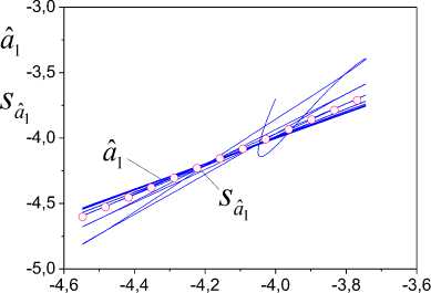
s :aˆ =0.6+1.14a , a1 1 1
raˆ21,a1 =0.95,
(78)
sˆ : aˆ = -0.002+a ,
raˆ22,a2 = 0.99,
(79)
where r2 , r2 are coefficients of determination mod- a1, a1 a2, a2
References Adaptive Observers with Uncertainty in Loop Tuning for Linear Time-Varying Dynamical Systems
- R.L. Carrol, D.P. Lindorff, "An adaptive observer for single-input single-output linear systems," IEEE Trans. Automat. Control, 1973, vol. AC-18. no. 5, pp. 428–435.
- R.L. Carrol, R.V. Monopoli, "Model reference adaptive control estimation and identification using only and output signals," Processings of IFAC 6th Word congress, Boston: Cembridge. 1975, part 1, pp. 58.3/1-58.3/10.
- G. Kreisselmeier, "A robust indirect adaptive control ap-proach," Int. J. Control, 1986, vol. 43, no. 1, pp. 161–175.
- P. Kudva, K.S. Narendra, "Synthesis of a adaptive observer using Lyapunov direct method," Jnt. J. Control, 1973, vol. 18, no. 4, Pp. 1201–1216.
- K.S. Narendra, P. Kudva, "Stable adaptive schemes for system: identification and control," IEEE Trans. on Syst., Man and Cybern, 1974, vol. SMC-4, no. 6, pp. 542–560.
- S. Nuyan, R.L. Carrol, "Minimal order arbitrarily fast adaptive observer and identifies," IEEE Trans. Automat. Control, 1979, vol. AC-24, no. 2, pp. 496–499.
- M.J Feiler; K.S. Narendra, "Simultaneous identification and control of time–varying systems," in Proceedings of the 45th IEEE Conference on Decision and Control, San Diego CA, U.S.A., 2006.
- Na Jing, Y. Juan, R. Xuemei, and G. Yu, "Robust adaptive estimation of nonlinear system with time-varying pa-rameters," International journal of adaptive control and signal processing, 2014, vol. 29, no. 8, pp. 1055–1072.
- G. Bastin, and M.R. Gevers, "Stable adaptive observers for nonlinear time-varying systems," IEEE Transactions on Automatic Control, 1988, vol. AC-33, no. 7, pp. 650-658.
- Y. Zhang, B. Fidan, and P.A. Ioannou, "Backstepping control of linear time-varying systems with known and unknown parameters," IEEE Trans. Automat. Contr., 2003, vol. AC-48, no. 11, pp. 1908–1925.
- Q. Zhang, and A. Clavel, "Adaptive observer with expo-nential forgetting factor for linear time varying systems," In Proceedings of the 40th IEEE Conference on Decision and Control (CDC ’01), December 2001, vol. 4, pp. 3886–3891.
- V.Ja. Katkovnik, V.Е. Heysin, "Adaptive control static essentially time-varying object," Automation and Remote Control, 1988, v. 49, no. 4, pp. 465–474.
- I.I. Perelman, "Methods of consistency estimation param-eters of linear dynamic objects and problematical character of their implementation on a finite sample," Automation and Remote Control, 1981, vol. 42, no. 3, pp. 309–313.
- D. Bestle, M. Zeitz, "Canonical form observer design for nonlinear time-variable systems." Int. J. Control, 1983, vol. 38, no. 2, pp. 419–431.
- J. Mason, E. Bai, L.-C. Fu, M. Bodson, and S. S. Sastry, "Analysis of adaptive identifiers in the presence of un-modeled dynamic: averaging and tuned parameters," IEEE Trans. Automat. Control, 1988, vol. AC-33, no. 10, pp. 969–979.
- N.N. Karabutov, "Identification of uncertain systems. I: Adaptive proportional-integral algorithms with uncertainty, "Automation and remote control, 1997, vol. 58, no. 11, pp. 1795-1805.
- A. Rodríguez, G. Quiroz, R. Femat, H.O. Méndez-Acosta, and J. de León, "An adaptive observer for operation moni-toring of anaerobic digestion wastewater treatment," Chemical Engineering Journal, 2015, vol. 269, pp. 186–193.
- N.N. Karabutov, "Identification of time-varying dynamic systems in space "input-exit", in Fundamental physical and mathematical problems and modeling of engineering-technological systems, 2004, is. 7, Publishing house "Ja-nus-K", pp. 209–218.
- K.S. Narendra, L.S. Valavani, "Stable adaptive controller design – direct control," IEEE Trans. Automat. Control, 1978, vol. AC-23, no. 4, pp. 570–583.
- N.N. Karabutov, Adaptive identification of systems. Mos-cow: URSS, 2007.
- E.A. Barbashin, Lyapunov function. Moscow: Nauka, 1970.
