Adaptive Path Tracking Mobile Robot Controller Based on Neural Networks and Novel Grass Root Optimization Algorithm

Published Online May 2017 in MECS DOI: 10.5815/ijisa.2017.05.01

Since the first launch of the Artificial Neural Networks (ANNs) and they have been used in many applications such as; image and signal processing [1], robotics control

[2], classification and clustering of data pattern sets [3]. The ANNs have the ability to approximate any nonlinear model by using parallel computation techniques [4]. One of the major topics related to the ANNs theory is the training process of the network weights. Many algorithms have been used for the learning purpose. However, one of the most famous algorithms in this field is the error back propagation algorithm which has been extensively used for the NNs training. Back propagation algorithm appears to be suffering from several problems such as easy being trapped into local minimum solution, and its low convergence speed [5]. Many papers have been proposed to develop the performance of the back propagation algorithm while other have just left this concept and migrate to another type of algorithms that called Metaheuristic Optimization Algorithms (MOA) [6,7] especially, in the training phase of the NNs.

The neural based controllers of robotic systems have been gained a great significance in the few recent years. These networks were recommended for their learning ability, adaptive behavior, and their high performance. An intelligent Mobile Robot (MR) has become an exciting choice for many scientific papers and industrial applications. Therefore, a lot of care have been spent to enhance controllers in the adaptive field and artificial intelligent.

This paper suggests an Adaptive Neural Controller (ANC), that's trained offline using MOA inspired by the grass plants reproduction and fibrous root system called Grass Root Optimization algorithm (GRO). The proposed ANC controller tracks the desired trajectory in the presence of parameters time variation and uncertainties using an offline fixed trained weight.

• II.    Related Works

  Many researchers have written to solve the problem of nonlinear trajectory tracking of wheeled mobile robot controllers under the conception of non-holonomic constraints. In 1995 R. Fierro and F. L. Lewis [8] propose an expanding for Kanayama tracking rule. The expanding

  integrates the kinematic controller with NN computed torque controller for the non-holonomic mobile robot. The proposed controller was designed to have the ability to deal with the basic non-holonomic MR and especially trajectory tracking problem, path following problem. In 2005 X. Jiang and et. al [9] proposed a mixed predictive and fuzzy logic mobile robot trajectory tracking controller. Fuzzy logic was intended to deal with the system nonlinear characteristic, while the predictive controller minimizes the time delay due to sensors low response, by predicting the position and direction of the MR. In 2012 R. M. Soto and et. al [10] used a hybrid evolutionary PSO and GA population-based optimization algorithm to design a fuzzy controller for the trajectory tracking of the MR. The hybrid evolutionary algorithm has been used to find the fuzzy membership function parameters. Both PSO and GA algorithms have to communicate with each other every predefined iteration number. In 2013 C. Raim Undez and A. Barreiro Blas [11] proposed an adaptive NN controller to compute the proportional torque besides another derivative to lead a non-holonomic MR through tracking problem. A dynamic inverse NN controller is responsible for the tracking trajectory, reduction of the obtained error and adaptation of the disturbance.

This work proposes a novel metaheuristic algorithm using it in optimization weights of ANNs that tracks the velocities and posture of a differential drive wheeled mobile robot in the presence of time variation of system parameters.

• III.    Grass Root Optimization Algorithm

Grass plants have three types of roots; primary roots, secondary roots, and hair roots. The first root grown in the soil is the primary root, which supplies the required energy and minerals to the first few generated leafs. Primary root is usually stayed active for only short time, till the secondary roots became active, then primary root dies and the new generated secondary roots take its function. The new initiated secondary roots develop new tillers and shoots and compete with other neighbor plant roots to absorb water and other minerals. On the other hand, hair roots are small branches, grow out of the epidermis of the secondary roots, they absorb almost all the required water and minerals. Grass plants have two major asexual reproduction methods. These methods usually depend on the stems that grow sideways; either under or above the ground. The first vegetative reproduction method in grass plants are the stolons, which are stems creep along the ground, while the second vegetative method is the rhizomes, which are stems grow below ground. Grass plants use both stolons and rhizomes to establish new grass culms. These stolons and rhizomes support the newly created grass plant until it became strong enough to live on its own [12].

Grasses perform global and local search to find better resources by reproduction of new grass plants using stolons and rhizomes and by developing their own root system. The generated new grasses and roots are developed randomly, but when grass arrives at a place with high resources, it generates more secondary roots, rhizomes, and stolons. The GRO algorithm depends the same reproduction and development of grasses to execute the global and local search. The algorithm starts by initializing random grasses in the search space, evaluates their fitness, generates a new population that contains the best-obtained grass and modifies its secondary and hair roots to search for better resources. If grass plant trapped into local minimum position, it generates new grasses by stolons initiated from the best-obtained grass, and other survived grasses. However, new secondary roots with different deviation from the local minimum solution will be generated by rhizomes. These roots help the trapped plant to reach farther places and escape the local position. GRO algorithm begins with an initial random uniformly distributed population (p) in the problem search space. The number of the initially generated grasses equal to the population size (ps). When iteration (it) begins, a new grass population (NP) is created. NP consists of three elements which are; the best grass obtained so far by the iteration process (gb = min(F (p))  RDim) where F is the cost function, Dim is the problem dimension. The second element of NP is a number (Gr) of grasses evaluated as in (1) and deviated from gb by stolons (SG) as in (2). These stolons deviated from the original grass with step size usually less than maximum upper limit vector ul. The last element of NP was a number of grasses equal to (ps–Gr-1) deviated randomly from the survived grasses of the iteration process (SD) as shown in (3).

Gr =

amse     i ( ps amse + minm Л 2

SG = ones ( Gr ,1 ) * gb + 2* max ( ul ) ... ...* ( rand ( Gr ,1 ) - 0.5 ) * gb

SD = GS + 2* max ( ul ) *...

... ( rand ( ps - Gr - 1,1 ) - 0.5 ) * ul

where amse is the average value of the mse vector shown in (4). mse i is the MSE value of i^th iteration given by (5), minm is the minimum of mse shown in (6). Ones( a ,1) is a column vector operator of a rows of ones. rand( a ,1) is a random column vector operator with a rows, its elements e [ 0,1 ] . max(.) and min(.) represent operators that find the maximum and minimum element of a vector respectively. GS is the ( ps-Gr-1 ) highest mse grasses retrieved from the last iteration process.

ps amse =      mse.

Ps £ no msei =— У(dsj - y j )2 no j =1

minm = min ( mse )

mse = 1 mse, ,..., mse, , ..., mse_n, ps

ds _j , y _j are the desired and actual values of the j^th output. (8) shows the new population vector NP .

NP = [ gb T SG T SD T ] T             (8)

Generated ( NP ) will be bounded and checked to get the fittest obtained grass. If the fittest new generated grass is best than the old one then keep the fittest new grass as the best grass solution. Otherwise, calculate the absolute rate of decrease in mse between the best grass obtained so far bestm shown in (9) and the current iteration minimum mse ( minm ) shown in (6). If the rate is less or equal a tolerance value ( tol ) shown in condition (10) increase global stack ( GC ) counter by one till it reached its maximum value then move to the local search mechanism.

bestm =min ( minm )              (9)

minm j - best m

minmj

< tol

minm= [ minm 1,.., minm j ,..,minm it ]^T           (11)

The local search mechanism consists of two individual loops; secondary roots loop, and hair roots loop. Hair roots are considered equal to the dimensions of the objective function ( Dim ), and each secondary root generated by the gb primary root represents a local candidate solution. The secondary roots number is represented by a random number usually less than Dim . Each single hair root modifies its location as in (12) for a repeated loops equal or less than secondary roots number ( SC ).

mgb k ^{+ 1} = agb + gb K + C 2 * ( rand - 0.5 )

k=1,2,…,SC and i=1,2,…,Dim.

Dim agb =---V mgbi

Dim       i

I = 1

C=[0.02,0.02,0.02,0.2,0.2,2,2,2,2,15](14)

C2=C(1+ rand *10)(15)

Where mgb is the locally modified gb, agb is the average of the mgb vector shown in (13), SC is the number of secondarily generated roots where (0 ≤SC≤ Dim), and C is the searching step vector shown in (14). C2 represents the random element of C chosen according to the percentage repetition of C elements as shown in (15). If the evaluated fitness of mgb is less than bestm then save gb as mgb. Otherwise, calculate the absolute rate of decrease in mean square error. If the rate is less than tol then increase local stack counter (CL) by one. When CL reached its maximum predefined value, break hair root loop and begin new secondary root loop. After each completed iteration check if the stopping condition (GE) is satisfied then stop the iteration. Otherwise, go to the next iteration until reached the mit (maximum iteration number) then stop. Table 1. illustrates the general proposed algorithm pseudo code.

• Table 1. GRO pseudo code

47:	Break For j
48:	End If
49:	End For ( j loop)
50:	End For ( q loop)
51:	End If
52:	End If
53:	If bestm ≤ GE then
54:	break For (it loop)
55:	End If

56:  End For ( it loop)

• A. GRO Optimizing NN Weights

The role of GRO algorithm is firstly; to bound and check the candidate solutions in population, modifies the solutions in an iteration process to get the best fitness solution. However, for supervised training NNs, the objective function is the Mean Square Error (MSE) function. Therefore, when the weights of the network are fully optimized, very minimum or zero MSE is obtained.

In order to make population-based metaheuristic GRO algorithm as a supervised training algorithm, we have considered all layer weights of the NNs as a grass vector in the population matrix. Each grass represents a candidate weight solution. The purpose of this weights vector is to minimize the objective MSE function of the NN. A number of weights in each grass vector represents the problem dimensions. Initial weights were created randomly, and the search space of the problem was limited to a minimum and maximum search space values.

Suppose the input data set represented by x ( M , ni ), and Ф (M , no ) is the target teacher. Where x E R ( ^M * ⁿ i ) and Ф E R ( M*no ), m i_s the number of input patterns, ni and no are the number of input and output neurons respectively. If we suppose that l is the hidden neurons number, then NN dimension with bias connections is represented by (16) for single hidden layer.

N =(ni * I +I) + (I * no + no)

For multiple hidden layers suppose that l is a vector represents the layers and neurons as shown in (17). The network total dimension is represented by (18).

l =[10 11 ^ lk . - 1m ], where 10 = ni, and 1m = no(17)

m - 1

N = Z( 1k +1) 1k+1

k = 0

Let the total weight vector Wt e R N , then the layer weight vector could be represented by (19), where i represents the layer number and N _i shown in (20) represents each layer number of neurons.

Wti =\ Wt N -v +^,-1 + 2 - Wt N i ] (19)

Approximately for most of the problems, a single hidden layer is usually sufficient to get the optimum solution. Two hidden layers are required sometimes for processing data with discontinuities and it rarely improves the performance of the networks. However, it may converge to a local minima solution when a large number of neurons is used. Therefore, there is no theoretical reason to use more than two hidden layers [13]. Hence, the network will have only two weights layer; input to hidden layer; and hidden to the output layer. For this purpose (19) will be rewritten as follows:

W1 =[wtx wt2--wtni*1+1 ]

W 2 = [ Wtni *1+,+1 Wtni *1+1+2._. wtN ]

Bi = [bi * ones (M ,1)]

ones (M ,1) = [11  12  -  1 m f(24)

Where W1 and W2 are the input to hidden weights layer and the hidden to output hidden layer respectively. Reshape W1 and W2 vectors into layer matrix form, then they will be written as follows:

	wt 1	wt 2   ^	wt l
Q =	wt 1 + 1	wtl +2  -	wt 2* 1
	wt ni * 1 + 1	wt ni * 1 + 2   • •	•   Wt 1 * ( ni + 1 )	(25)
	Qn	Q 12   —	Q 1 1
=	Q 21	Q 22   —	Q 2 1
	^ ( ni + 1 ) 1	Q( ni + 1 ) 2   •	Q( ni + 1 ) 1

^ =	Wt 1 * ( ni + 1 ) + 1      — Wt I * ( ni + 1 ) + no + 1    • Wt 1 ( ni + 1 + no ) + 1    —			Wtl * ( ni + 1 ) + no Wtl * ( ni + 1 ) + 2 no Wt I ( ni + 1 + no ) + no		(26)
		^ 11	^ 12   •	V 1 no
	=	^ 21	^ 22   •	••      Y 2 no
		_ ^ ( I + 1 ) 1	^ ( I + 1 ) 2	-  ^ ( 1 + 1 ) no _

N i =

■ ( 1 i + 1 ) 1 i _{+ 1}, fori >  0

0, fori <  0

Where Q e R ^{( n}i ^{+ 1 ) 1} , and ^ e R ^{( 1 + 1 ) no}

Xb = [Bi x](27)

Xb g R Dm ⁽ ni ^{+ 1 )} is the input pattern data set with input bias. The hidden layer output is shown in (28) for linear activation function.

h = Xb*Ω(28)

Where h g R Dm*l . Adding bias to (28), another vector is constructed as in (29). The output of the network is shown in (30) for linear identity function.

H = [ Bi h](29)

y = H *^(30)

Where H g R Dm * ⁽ l ^{+ 1 )} , y G R Dim * no

^p =

cos ( S )   0

sin ( S )   0

Λ

For non-slipping and pure rolling condition, the non-holonomic constraint is shown in (35) [8].

Xsin ( S ) - Ycos ( S ) = 0             (35)

IV. Differential Drive Wheeled Mobile Robot

For the kinematic and dynamic MR modeling, suppose the model proposed by [14]. Fig. 1 shows a general differential drive wheeled MR geometrical structure, in which the point B represents the central point between the driver wheels, b is the straight distance between the center of gravity A and the wheel axis. The MR position is described by p = [ X, Y, z5]^T, where X , and Y are the axis of point A. 1 is the mobile robot steering rotation angle. The MR kinematic model is given by (31-33).

Let m be the mass of the robot platform, m m the mass of the wheel and motor, I is the moment of inertia of the robot platform about the perpendicular axis over B, I m is the wheel and motor moment of inertia around the wheel axis, and I i is the wheel and motor moment of inertia around the wheel diameter. The dynamic robot model is represented by equations (36-41) as follows:

M ( p ) Л + N ^ p ,p ^ Л = B ( p ) т         (36)

Where ^т =[ ^T _r, ^T l ] stand for the right and left torques applied on the wheels, while M , N , B are represented by:

M ( p ) =

-j ^ ( mb ² + I_t ) + Im 4 d ²

4 d T ^{( m}b ² - It )

4^ ( mb¹ - I )

X- ( mtb ^{2 +} It ) ⁺ Im )

4 d ²

^p = Q ( p ) ^ф

Where Ф =[Ф_г, Ф 1 ]^т, are the right angular velocities.

and

left wheels

r ²

— ( mbw )

Q ( p )=

j cos ( ^S ) rsin ( ^S )

j cos ( S ) ^sin ^{( s )}

d

—d

Ф =

b

b

—

Л = [ v, w ]^T represents the linear and angular velocities of the wheeled MR. Substituting (32) and (33) in (31) obtains the kinematic system model of the differential drive robot in terms of linear and angular velocities as shown in (34).

r ²

-Чд ( mbw )

B =

Where I t , and m t represent the total moment of inertia and the total mobile robot mass as in (40-41).

I_t = mb ² + 1 + 2 m m d ² + 2 I i          (40)

m_t = m +2 m m               (41)

V. The Proposed ANC

This paper develops a trajectory tracking controller based on NNs that has been optimized using GRO algorithm for the differential drive MR of the Fig. 1. We have assumed that there is uncertainty in the dynamic system model. Furthermore, distance b, platform mass m , wheel radius r , and the platform width c l are varying with time. After the NN training phase finished, the controller considered to be tough against parameters variation and

tracks the proposed trajectory at the dynamical and kinematic controller levels.

The control inputs V and W which make E 1 , E 2 , E 3 converge to zero are given by (44) [15].

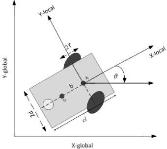
Fig.1. Differential Drive wheeled MR geometrical structure.

If supposed that there is a predefined desired trajectory given by (42).

P d =

cos (Sd)  0

sin (^S d )   0

Where P d =[ X d , Y d , ^S d J , ^л а =[ v d ,w d ] . The error between the desired and actual pose in the local robot frame are given by:

E 1

E

E

= T

e ₁

e ₂

cos ( S ) sin ( S )

- sin ( S )   cos ( S )

0 X d - X

Y d — Y

V

W

cos ( E₃ ) kyE 2

vd wd

k_xE ₁ k _s sin ( E з )

Where k x , k y , k_fl > 0, represent the positive constants.

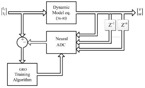
Fig.2. The NDC training phase

The DNC is designed to learn the collected input/output data from the dynamic model system (36-41) and learns the torque signals which transfers the MR from velocity at time ( t ) to upcoming ( t+1 ) velocity. The DNC offers, after good training, an adaptive performance with fixed trained weights. However, the DNC has to be well trained for all possible parameters variation of the dynamical model especially, the values b, m , c l , and r . Fig. 2 shows the DNC training phase block.

e ₃

i L S _d - s

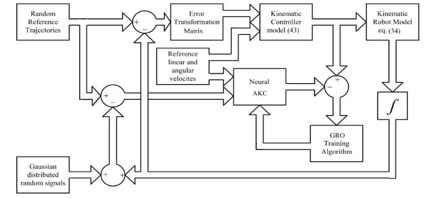
Fig.3. The KNC training phase.

The robot nominal values are proposed as follows; r = 0.033 m, m = 0.575 Kg, c l = 0.15m, b = 0.04 m. While for the training of the DNC purpose, we assumed that m varied between the values [0.45 , 1.2] Kg, distance b is varied in the interval of [0.03, 0.1] m, cl varied in between [0.12, 0.2]m, r varies between [0.03, 0.07] m.

The training torques input data are proposed randomly uniformly distributed in between [-0.01,0.01] N.m. On the other hand, the KNC is proposed to learn the behavior of the backstepping feedback controller system (44) and to raise its robustness against disturbance data. For the purpose of training the KNC, A random trajectory ρr was created, and a noisy data having zero mean and 0.1 variation level Gaussian distributed was added to the training data. The training input data of the KNC were the randomly created trajectory reference velocities and the error between the random trajectory and the kinematic model trajectory output plus noisy Gaussian distributed data. Fig. 3 shows the KNC training phase block.

10,000 samples data sets have been generated. These patterns data sets were divided into two sub-data; 5000 sets for training purpose, and 5000 sets for testing of the trained network. The used NNs architecture of both DNC and KNC consisted of single hidden layer with 4 hidden processing neurons and 2 output neurons. The DNC has 4 input neurons for the desired and real velocities, while KNC has 5 input neurons for the random reference velocities and the error posture with disturbance. The synaptic weights connections were randomly initialized between [ - 1 , +1]. Linear identity activation function has been used for both input and hidden layers. 10 training cycles have been executed for both DNC and KNC. Each training cycle has 1000 maximum iterations (mit). 30

grass population (ps) were used . GRO algorithm stops iterations according to three proposed stopping conditions which are:

• ❖    If any grass converged to the predefined global error value, which is zero MSE in our case.

• ❖    When the testing MSE exceeds the training MSE by10% of its value.

• ❖    When the algorithm completes the whole iteration cycles.

If GRO finished a training cycle without overfitting, the next cycle continues from the last reached point of the last valid cycle. The network weights will be the last known valid weights. The overall ANC structure is shown in Fig. 4. It consists of two feedback control loops; external feedback KNC controller that generates the control velocity signals that tracks the desired trajectories, and DNC internal control loop which is designed to improve the controller robustness against parameters uncertainty and time variations.

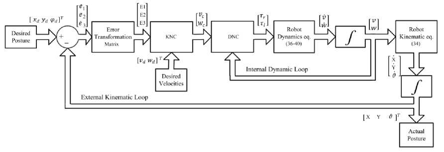
Fig.4. Overall ANC block diagram

Table 2. Dynamic parameters time variations.

Parameters	nominal values	Maximum values	Minimum values
b (m)	0.04 m	0.14 m	0 m
cl(m)	0.15 m	0.5 m	0.1 m
r (m)	0.033 m	0.093 m	0.023 m
m (Kg)	0.575Kg	3 Kg	0.25 Kg

The desired velocities generated for the path tracking are illustrated in Table 3. The desired posture is found by integrating (34).

For the purpose of testing the wheeled MR tracking performance, the mobile robot parameters have been assumed varying randomly as illustrated in Table 2. The MSE of the MR position and velocities are evaluated by (45) and (46).

Table 3. velocities trajectories.

t	v d	w d
0 < t < 157	Г      Г 2t 0.05 1 - cos — (      ( 10 J J	0.05 1 1 - cos| — 1 1 I      1 10 JJ
157.1 <  t <  300	0.05 1 - cos| — | (      ( 10 JJ	Г           ^ - 0.05 1 - cos — (       (10 J J

Erp = 1V E 12 + E 22 + E 3

Errv

2 (v^

- v ) ^{2 +} ( w d - w ) ²

The GRO algorithm first training cycle for KNC and DNC are shown in Fig. 5 and Fig. 6 respectively. After 10 training cycles without overfitting of the KNC. The recorded maximum MSE was 0.0002 for the linear velocity and 0.4221 for the angular velocity. The average angular and linear velocities MSE was 0.2112 which is relatively high MSE, due to the large set of training input sets. The average testing MSE was 0.2042.

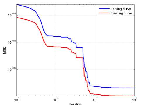
Fig.5. First epoch GRO training algorithm MSE for the KNC.

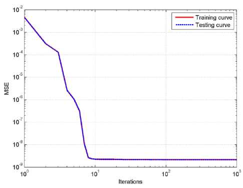
Fig.6. First epoch GRO training algorithm MSE for the DNC.

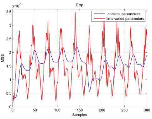
Fig.7. Mobile robot Errp MSE.

For the second DNC network, the recorded MSE was 2.33e-10 for the left torque signal and 2.07e-10 for the right torque signal. The average MSE of both torques was equal 2.199e-10 with testing average MSE of 2.124e-10. This very minimum value actually is due to the tiny torque signals that have a maximum value of 0.0001 N.m. The mobile robot position MSE (Errp) and velocities

MSE (Errv ) were shown in Fig. 7 and Fig. 8. The velocity and position MSE of the MR with nominal parameters and time-varying parameters are less than 3.5e-03. Finally, Fig. 9 shows the real and desired x-y trajectories tracking.

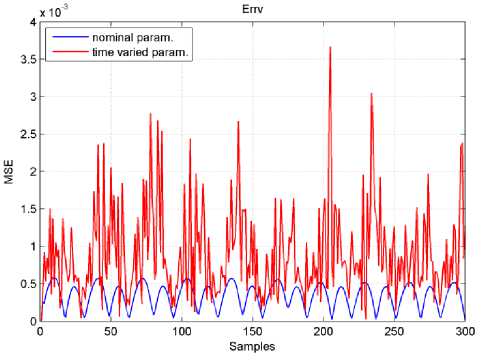
Fig.8. M obile robot E RRV MSE.

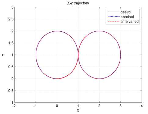
Fig.9. X-Y trajectory tracking.

• VII. Conclusions

This paper proposes novel GRO algorithm optimizing an inverse ANC trajectory tracking wheeled MR. ANC consists of two subs NNs; KNC and DNC using internal and external feedback loops. The internal DNC feedback loop makes the robot more robust against parameters uncertainty and parameter time variations, while the external KNC responsible for tracking the desired angular and linear velocities of the MR and the posture x, y, and 6.

Both NNs trained using GRO algorithm. Applying 10 iteration cycles each with 1000 maximum iterations for both of networks. Fig.7 and Fig. 8 have shown the position and velocity MSE, from these figures we notice that the controller succeeds in tracking the MR under fixed nominal and time varying parameters. The ANC performance generally didn't effect by the parameters variation even when some parameters increased by more than 300%. Therefore, this controller has shown a great performance against parameters variation with only 8 hidden neurons for both KNC and DNC without any overfitting during data training process using the GRO algorithm. Although we have used large training and testing datasets, there was no data overfitting, this is due to the used techniques of observing the training and testing data at the same time. Since the training was offline and have been carried only once (10 cycles) GRO processing time has not been taken into consideration.

• [1]    K. H. Teng, T. Wu, Z. Yang, C. H. Heng and X. Liu, "A 400-MHz wireless neural signal processing IC with 625 on-chip data reduction and reconfigurable BFSK/QPSK transmitter based on sequential injection locking," 2015 IEEE Asian Solid-State Circuits Conference (A-SSCC) , Xiamen, pp. 1-4, 2015.

• [2]    Neha Kapoor, Jyoti Ohri,"Evolutionary Optimized Neural Network (EONN) Based Motion Control of Manipulator", International Journal of Intelligent Systems and Applications IJISA , vol.6, no.12, pp.10-16, 2014.

• [3]    Yevgeniy Bodyanskiy, Olena Vynokurova, Volodymyr Savvo, Tatiana Tverdokhlib, Pavlo Mulesa,"Hybrid Clustering-Classification Neural Network in the Medical Diagnostics of the Reactive Arthritis", International Journal of Intelligent Systems and Applications (IJISA), Vol.8, No.8, pp.1-9, 2016.

• [4]    R. Murugadoss and M. Ramakrishnan, "Universal approximation of nonlinear system predictions in sigmoid activation    functions using    artificial neural

  networks," 2014 IEEE International Conference on Computational Intelligence and Computing Research , Coimbatore, pp. 1-6, 2014.

• [5]    S. Chai and Y. Zhou, "A Study on How to Help Back-propagation Escape Local Minimum," Third International Conference on Natural Computation (ICNC 2007) , Haikou, pp. 64-68, 2007.

• [6]    Koffka Khan,Ashok Sahai,"A Comparison of BA, GA, PSO, BP and LM for Training Feed forward Neural Networks in e-Learning Context", International Journal of Intelligent Systems and Applications IJISA , vol.4, no.7, pp.23-29, 2012.

• [7]    Hanan A. R. Akkar, Firas R. Mahdi, “Training ArtificialNeural Networks by PSO to Perform Digital Circuits Using Xilinx FPGA,” Eng. & Tech. Journal , Vol. 29, No. 7 pp. 1329-1344, 2011.

• [8]    R. Fierro and F. Lewis, “Control of a Nonholonomic Mobile Robot Using Neural Networks,” IEEE Transactions on neural networks , vol. 9, pp. 589–600, 1998.

• [9]    X. Jiang, Y. Motai and X. Zhu, "Predictive Fuzzy Logic Controller for Trajectory Tracking of a Mobile Robot," Proceedings of the IEEE Midnight-Summer Workshop on Soft Computing in Industrial Applications. SMCia/05. , pp. 29-32, 2005.

• [10]    R. Martinez-Soto, O. Castillo, L. T. Aguilar and I. S. Baruch, "Bio-Inspired Optimization of Fuzzy Logic Controllers for Autonomous Mobile Robots," Fuzzy Information Processing Society (NAFIPS), Annual Meeting of the North American , Berkeley, CA, pp. 1-6, 2012.

• [11]    Raimúndez and A. B. Blas, "Adaptive Tracking in Mobile Robots with Input-Output Linearization," Industrial

  Electronics Society, IECON 39^th Annual Conference of the IEEE , Vienna, pp. 3299-3304, 2013.

• [13]    Gaurang Panchal, Amit Ganatra, Y P Kosta and Devyani Panchal, "Behaviour Analysis of Multilayer Perceptrons with Multiple Hidden Neurons and Hidden Layers," International Journal of Computer Theory and Engineering, Vol. 3, No. 2, April 2011.

• [14]    T. Fukao, H. Nakagawa, “Adaptive Tracking Control of a Nonholonomic Mobile Robot,” IEEE transactions on Robotics and Automation , vol. 16, pp. 609–615, 2000.

• [15]    Kolmanovsky and N. H. McClamroch, "Developments in nonholonomic control problems," in IEEE Control Systems , vol. 15, no. 6, pp. 20-36, Dec 1995.