Aerodynamic System Modeling based on Proper Orthogonal Decomposition

Published Online November 2011 in MECS

A Reduced order model is any low-order model that retains the characteristics and dynamics of the original system. It has been applied throughout many different disciplines, including controls, fluid dynamics, and structural dynamics. One of the most popular methods for model order reduction is proper orthogonal decomposition. The proper orthogonal decomposition (POD) is known as Karhunen Loéve expansion and principle components analysis. As an effective method for data analysis, the POD methodology has been widely used for a broad range of applications, including reduced order model (ROM) construction, data reconstruction, image processing and pattern recognition[1~7].

For aerodynamic inverse design problems, Everson and Sirovich have developed a modification of the basic POD method that handles incomplete data sets. Given a set of POD modes, and incomplete data vector can be reconstructed by solving a small linear system. This method has been successfully applied for reconstruction of images, such as human faces, from partial data.

Manuscript received April 10, 2011; revised June 8, 2011; accepted May 5, 2011.

For aeroelastic problems, with the recently well-developed software and hardware, (CFD)-based, nonlinear aeroelastic simulation capabilities have shown that for low to moderate angles of attack, they can be a reliable alternative to linear theories, However, the high fidelity models generally result in very large computational domain easily involving at least 105 and usually greater than 106 degrees of freedom (DOFs). Because of this computational cost, the potential of CFD-based nonlinear aeroelastic codes is currently limited to the analysis of a few, carefully chosen configuration rather than routine analyses. In response to this challenge, in recent years, substantial research has been conducted in developing reduced order models (ROMs) of highdimensional CFD models with the goal of reducing computational time by orders of magnitude[8~13]. For conventional POD method, only system inputs characteristic has been considered. Without consideration of the relationship between outputs and system states, inefficient models may be obtained, and the higher degrees of ROM could be achieved. A reduction procedure based only on system inputs may be highly dependent on the arbitrary scaling of the states variables, and it could lead to reduced models that are highly inaccurate.

In this paper, the basic POD approach is firstly outlined, followed by the description of POD based inverse-design methodology. Airfoil flow field inverse design cases demonstrate the accuracy of POD method. Finally, balanced modification is introduced in POD method for reduced order model construction. Aeroelastic structure active control case indicates POD method with balanced truncation is efficient and accurate for real aeroelastic analysis.

• II.    Proper Orthogonal Decomposition (POD)

The basic idea of POD is to obtain the optimal subspace with order m by using sample data (snapshot) x^k derived from n order data space ( m < n ). The n order space is projected onto the optimal subspace to extract POD modes. The error between ROM and full order system is defined as:

G = min]T|| x^k - 0r ‘ || , x k e C N , Q = Ф-Ф ^H (1) ^Ф k = 1

The equation (1) which represents min-problem can be transferred into a max-problem. That is:

H = max t ⁽ x ^k , ^Ф) , Ф H Ф= I (2) ^Ф - hl Г

The constrained optimization is performed via standard optimization techniques where a Lagrangian function is constructed as shown below:

m

J W= l ( ( x k , Ф ) ) - а (|Ф| Г — 1 )             (3)

The differentiation of equation with respect to Φ leads to the following:

—J (Ф) = 2 XXT Ф-2АФ d Ф V 7                            (4)

For large systems, the matrix R=XX^T (POD kernel) will be of a very large dimension n × n , if the data ensemble consists of m< linearly independent data samples, the following equivalent, smaller, m×m eigen problem can be solved instead.

X T X Y = ФЛ              (5)

The non-zero eigen spectrum of the two systems are the same, and the eigenvectors are related via the snapshot matrix X, so that

" 1

Ф = X ^Л" ²                 (6)

Model reduction using the POD basis is accomplished by truncating the number of eigenvectors, also known as POD vectors. The singular values are often referred to as the “energy” contained in the system, and physical significance maybe attributable to these singular values. Generally, truncation of the POD vectors is done so that the ratio of total energy in the reduced subspace energy in the full order space is close to one or

r

I А-

=И— « 1.

m

I А

I = 1

to the

The proper orthogonal decomposition can therefore be summarized as follows:

• (1)    Collect snapshots of primary system to construct matrix X.

• (2)    Obtain the eigenvectors of the correlation matrix X^TX to determine POD kernel.

• (3)    Retain only those eigenvectors in the reduced space basis that correspond to large Hankel singular values.

• III.    POD for Inverse Design

Inverse design vector in terms of p POD basis functions can be described as:

g = 1 л ф ,

•=1

The error E between the original and inverse design vectors is defined as

E = 1 g — g I(9)

The coefficients b can be solved by differentiating Eq. (9) with respect to each of the b . This leads to the linear system of equations

Mb = f(10)

Where M j = (Φ i , Φ i ) n and f i =(g, Φ i ) n

Solving Eq. (10) for b and inverse design vector g can be obtained.

A Cases Val dat on

The case considered is the RAE 2822 airfoil at a free-stream Mach number of 0.5 with grid size 121×33. To create the POD basis, 26 snapshots are computed at uniformly spaced values of angle of attack in the interval а = [-1.25°, 1.25°] with a step of 0.1°. As shown in Fig.1, we see that magnitudes of eigenvalues drop off very quickly, indicating that the reduced order model will quite only a few states. In fact, the first 3 contains almost 99.99% of the system “energy”.

10-5

А

p

E А

¹   10^-10-

10-15

□

Ч^п

A^

0       5      10      15      20      25      30

POD modes

Fig1. Distribution of singular values

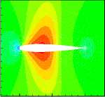
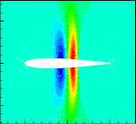
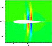
An incomplete flow-field was then generated by computing the flow solution at a =1.2° (which is not one of the snapshots), and then retaining only the pressure values on the surface of the airfoil. The total number of pressure values in the full flow-field is 3993 and the number of pressure values on the airfoil is 121, hence 96.97% of the data is missing. The main goal, then, is to design the full pressure flow-field using POD method introduced in recent paper. Such a problem might occur, for example, when analyzing experimental data. Typically, experimental measurements will provide only the airfoil surface pressure distribution. The POD method provides a way to combine this experimental data with computational results in order to inverse design the entire flow field. Fig.2 (1) and (2) show the pressure contour of the first two POD modes.

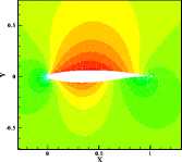
(1) 1st POD mode

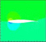
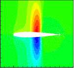
(2) 2nd POD mode

Fig2. Pressure distribution of the first 2 POD modes

Fig.3 shows the inverse designed pressure contour with 3 POD modes, compared with the original contours of the CFD solution. With just limited surface pressure data available, the complete pressure field can be determined very accurately with only 3 POD modes, showing that the POD methodology for data construction works effectively for aerodynamic application.

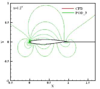
Fig.3 Interpolation pressure comparison

Another example is for α =1.5° and α =2.0°, which are not within [-1.25°, 1.25°]. As shown in Fig.4 (1) and (2), the POD method also predicted original pressure contour accurately. But for α =2.5°, the result is not reliable, even if more POD modes are used. The above results show that POD method allows models to be derived that accurately predict steady-state pressure fields either by interpolation or extrapolation. The approach can also be extended to other flow parameters such as temperature or density field.

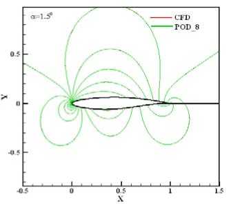
(1) α=1.5°

Cases shown above are subsonic flow around RAE 2822 airfoil. The POD methodology also is used for transonic flow case. The case considered is the NACA 0012 airfoil at a free-stream Mach number of 0.8 with grid size 121×33. The POD bases are created in the same way as RAE 2822 case. As shown in Fig.5, we see that magnitudes of eigenvalues drop off very quickly, indicating that the reduced order model will quite only a few states. In fact, the first 6 contains almost 99.87% of the system “energy”. Fig.6 shows the pressure contour of the first 6 POD modes.

Fig.7 shows the reconstructed pressure contour with 6 POD modes, compared with the original contours of the CFD solution. The complete pressure field can be determined very accurately with 6 POD modes, showing that the POD methodology for data construction works effectively for transonic flow, in which the shock wave presents.

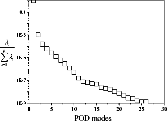
Fig5. Distribution of singular values

(1) 1st POD mode

(2) 2nd POD mode

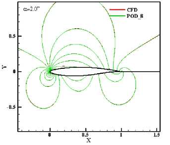
(2) α=2.0°

Fig.4 Extrapolation pressure comparison

(3) 3rd POD mode

(4) 4th POD mode

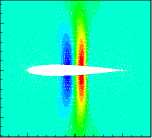
(5) 5th POD mode

0.5

-0.5

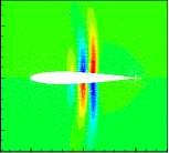
(6) 6th POD mode

Fig6. Pressure distribution of the first 6 POD modes

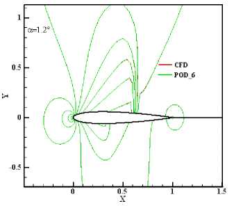
Fig7. Inverse design by 6 POD modes at a — 1.2°

IV.    POD with Balanced Modification

For conventional POD method, only system inputs characteristic have been taken into account, without consideration of the relationship between outputs and system states. Therefore, the robustness of POD based ROM cannot be guaranteed. POD method with balanced modification is introduced in this section. The outline idea of modified POD method is to construct POD kernel with snapshots of primary system and dual system.

Consider an n order state-space system and its dual system defined in (11), (12)

X = Ax + Bu y = Cx                      (Ц)

z = ATz + CTv w = BTz                        (12)

Excite the original and dual system with dirac delta signal and collect states vector to construct snapshots matrix X and Z. Then the POD kernel is update to R=ZTX. Therefore, the kernel R takes both input and output characteristic of original system into account. The new POD method can therefore be summarized as follows:

• (1)    Collect snapshots of primary system to construct matrix X.

• (2)    Collect snapshots of dual system to construct matrix Z.

• (3)    Obtain the eigenvectors of the correlation matrix Z^TX to determine POD kernel.

• (4)    Retain only those eigenvectors in the reduced space basis that correspond to large Hankel singular values.

• A.    Case Validation

Consider a typical 2D aero-servo-elastic system, which is illustrated in Fig.8. Detail structural parameter is in Ref [16].

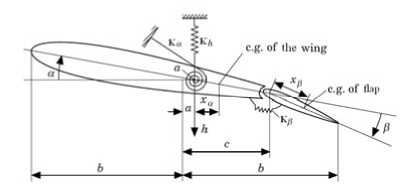
Fig.8 Schematic of airfoil section with control surface

The new POD method is used to construct ROM for Euler equation, which is repeated below.

— J Q d fi + |j F ■ ds = 0

⁵ t " ( t )           s ( t )                                   (13)

The inviscid flux is calculated using the AUSM+~up scheme. The 2nd order accuracy is obtained with MUSCL interpolation and Van Albada limiter. Deforming mesh is achieved by using the TFI method. Euler code is validated through AGARD test CT5 [14]. The results shown in Figure 9 are in good agreement with experiment data.

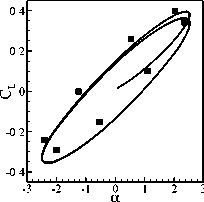
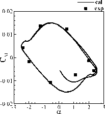
Fig.9 Comparison between calculation and experiment

• B.    Full Order state space model (FOM)

Euler equation can be described as shown below:

( Aw ) t + F ( w, u , v ) = 0

Here, A is the diagonal matrix of cell volumes, F is the nonlinear numerical flux function, and w is the conservative state vector, u is the structural displacement vector; v is the structural velocity vector; t represents a partial derivative with respect to time. Full order state space can be constructed though Taylor series expansion about given operation point W0.

Ao w , + Hw + ( E + C ) v + Gui = 0

и 6F              6F u

H = — (w , u , v ) G = — (w , u , v ) o o oo o o ow r dFd

C = —⁽ w o , ^u o , v o ) ^E = —w o

8 v

The matrices H, G, E, and C are the 1st order terms in a Taylor series expansion of the numerical flux function evaluated at the operating point. The matrix H is the gradient of the numerical flux function with respect to the fluid states and thus will be very large sparse matrix. The full order system is derived as:

w = A ■ w + B ■ y

G = P ■ w                   (16)

A = - A o ^{- 1} , B= - A o ^-1 ( G , E + C ) , y = [ u , v ] T

Matrix P represents force partial derivative with respect to w, and G is output force vector.

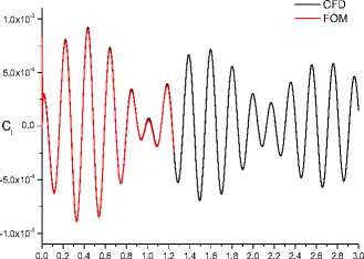
The O-type grid dimension is 121×31, shown in Fig.10, and the degree of the aerodynamic system is n=120×31×4=14400. Flow condition is described in Ref [16]. Results shown in Fig.11 indicate FOM reproduces faithfully the response predicted by CFD, and ready for POD-based ROM construction.

4.0x10-4

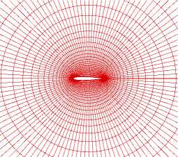
Fig.10 O-type grid for aero-elastic simulation

C. Reduced Order state space model (ROM)

Apply a dirac delta signal individually to each structural mode and collect 200 snapshots using a time step ⊿ t=5×10-4(s).Given that there are 2 displacement inputs and 2 velocity inputs, this resulted in a snapshot matrix X of primary system with 800 data samples. Collect snapshots of dual system and construct snapshot Z with 400 data samples. The snapshot matrix is used to form the correlation matrix R=Z^TX of dimension 400×800. The POD vectors are computed by computing the eigenvectors of R. Once the POD basis vectors are computed, the reduced order models are formed via projection resulting in the following reduced system. Given the reduced order m, then reduced system is of the dimension m×m (m<

w r = Ф J А Ф r w r + Ф J By

CFD

FOM

2.2 2.4 2.6 2.8 3.0

0.0 0.2 0.4 0.6 0.8 1.0 1.2 1.4 1.6 1.8 2.0 time(s)

F = Р Ф r w r

-4.0x10-4

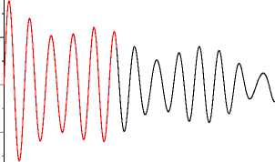
Fig.12 shows the eigenvalues of the first 80 proper orthogonal decomposition vectors. The spectrum of eigenvalues decay quickly, and the first 80 POD vectors contain the vast majority energy. 55th order ROM is constructed by truncating low energy modes. Results shown in Fig.13 suggest 55th ROM is accurate enough. The order of ROM is just approximately 4% of FOM.

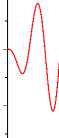
(1) Plunging response

CFD

FOM a 0.0

-1.0x10-4

1.0x10-4

0.00.20.40.60.81.01.21.41.61.82.02.22.42.62.83.0

time(s)

-2.0x10-4

(2) Pitching response

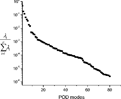
Fig.12 Hankel singular values

times(s)

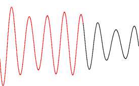
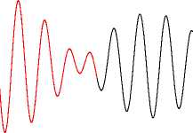
(3) Lift coefficient

Fig.11 FOM and CFD comparison

4.0x10-4

h/b

ROM_55 FOM

0.0

2.0x10-4

-2.0x10-4

0.0                 0.5                 1.0

time(s)

-4.0x10-4

ROM_55 FOM

1.0x10-4

a 0.0

-1.0x10-4

(1) Plunging response

0.0                 0.5                 1.0                 1.5                 2.0

time(s)

-2.0x10-4

(2) Pitching response

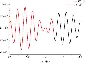
(3) Lift coefficient

Fig.13 FOM and ROM comparison

The LQR control method is employed for present aeroelastic structure active control. Coupled with 6th order structural model, 61th order aero-servo-elastic ROM was constructed for close loop analysis. The control plant is shown in Figure14.

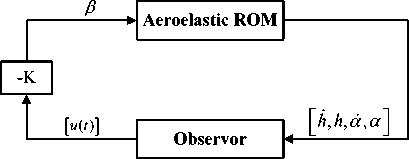
Figure14 Control plant with LQR

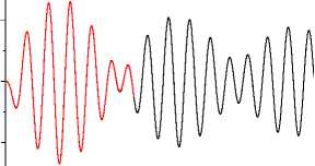
The control results shown in Figure15 indicate that the responses are suppressed quickly, with flap deflect angle -0.2° approximately. Additionally, the 61th order aeroservo-elastic ROM can be used for control law optimization efficiently with high fidelity compared with CFD direct calculation.

4.0x10-4

2.0x10-4

h/b

0.0

-2.0x10-4

a

FOM

ROM_55

-4.0x10-4

0.00.51.01.52.02.5 time(s)

(1) Plunging response

4.0x10-5

2.0x10-5

0.0

-2.0x10-5

FOM

ROM_55

-4.0x10-5

0.0             0.5             1.0             1.5             2.0             2.5

time(s)

(2) Pitching response

8.0x10-4

4.0x10-4

p

0.0

-4.0x10-4

-8.0x10-4

-1.2x10-3

0.0

0.5

1.0

1.5

2.0

time(s)

FOM

ROM_55

2.5

(3) Lift coefficient

Fig.15 Structural response with active control

V. Conclusion

POD method is presented in this paper for flow field inverse design. A new POD method with balanced modification is also introduced to improve robustness of conventional POD method for unsteady aerodynamic force ROM construction. The major computational cost is the computation of the snapshots, from which the vectors are extracted. However, once the vectors are obtained, the cost of constructing and solving the reduced order model

is negligible, allowing quickly performing parametric studies.

Airfoil flow field inverse design and 2D aero-servoelastic active control problems are chosen for method validation. All the results shown POD based ROM are much more efficient than CFD simulation without losing accuracy and the information of the nature full-order system.