Agent-based Modeling in doing Logic Programming in Fuzzy Hopfield Neural Network

The neural network is a parallel processing network, generated by the simulation of the intuitive thinking of the human’s image drawing upon exploring the biological neural network with regard to the biological neurons, as well as the features of the neural network through simplifying, summarizing, in addition to refining [1]. Moreover, the nonlinear mapping idea is utilized, the parallel processing method, in addition to the neural network’s structure for expressing the related knowledge of input, as well as the output [2]. The Hopfield model [3, 4] can be defined as a sole layer recursive neural network, whereby each neuron output can be associated with every other neuron input. Hopfield neural network’s energy function is a quadratic function, which is joined with the objective function so that the problems of optimization are minimized [5].

A method is introduced by Wan Abdullah [6] of performing a logic program in the Hopfield network. The network conducted a logical inconsistency minimization in a program after defining the connection strengths by a logic program, that is, through equating cost function, in addition to energy function. The network, after that, relaxes to the neural states, which are the models (i.e., viable logical interpretations) of the corresponding logic program. The direct method involves introduced learning by Wan Abdullah [7].

In this paper, the technique of the fuzzy Hopfield neural network clustering, combined with a modifying activation function, has been introduced with the aim of solving combinatorial optimization issues. Thus, the fuzzy Hopfield neural network involves a specific numerical procedure. It can minimize an energy function so that the membership grade is located [8]. Combinatorial optimization involves locating a set of options among a discrete set to provide the most optimum value of the corresponding cost function [9]. According to fuzzy Hopfield neural network, the algorithm of fuzzy c-means clustering has been imposed to activate the states of the neuron without exception in a Hopfield neural network. Accordingly, using the method of fuzzy Hopfield neural network clustering has been analyzed with the modification of an activation function to fast move computation to perform the logic programming in the given Hopfield network.

Furthermore, agent-based modeling for the proposed method is introduced in this paper. In FCMHNN, a unique Hopfield network was modified with the addition of fuzzy c-means clustering approach. The energy function, then, could be swiftly converged to local minimum. Compared to the conventional technique of HNN, the introduced FCMHNN fundamental strength showed more computation efficiency because of integral corresponding structures. Based on the simulation study, FCMHNN showed that it is capable of yielding promising results compared to HNN.

In the subsequent section of the paper, the focus is placed on the Hopfield neural network. Next, the paper investigates how logic learning has been carried out in the Hopfield network followed by explaining how fuzzy logic is integrated into the Hopfield network. After that, a discussion about agent-based modeling is provided. Finally, the conclusion of the study is provided in the last section of this paper.

2.    Hopfield Neural Network

The Hopfield Neural Network (HNN) provides a model that simulates human memory. It has a wide range of applications in artificial intelligence, such as machine learning, associative memory, pattern recognition, optimized calculation, VLSI and parallel realization of optical devices. The Hopfield model can be defined as a sole layer recursive neural network, whereby each neuron output can be associated with every other neuron input. The Hopfield network’s energy function, which is a specific quadratic function, can be connected to an objective function to reduce optimization issues.

The Hopfield network, involving n units, is having a couple of versions. These involve binary, in addition to the continuously valued. Consider v is a state or an output of i th unit. Regarding the binary networks, v denotes +1 or -1, however, regarding continuous networks, v denotes a specific value between 0 and 1. Consider w is synapse weight on the connections from units i to j . According to Hopfield networks, w = w. , V i , j (symmetric networks), as well as w^ = 0 , V i (i.e., no self-feedback connections). The dynamics of the network of the given binary Hopfield network involve:

v_f = sgn| ^ ^wy Vj — threshold (

The energy function of the discrete Hopfield network can be provided by:

E =-- V V w.v.v. - V w.v.

ij i j                   i i

2i j                       j ij        j

Fig.1 shows the discrete Hopfield network as the extended form of the common representation of the given Hopfield network. In Hopfield and Tank’s work [3], the network can be usefully utilized to solve problems of combinatorial optimization as a content addressable memory or as an analog computer. Thus, combinatorial optimization is to locate a set of options from a given distinct set that can produce the best value of several connected cost function.

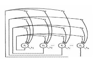
Fig. 1. Discrete Hopfield neural network

Because the network progresses based on the dynamics, a given energy E can be decreased only or remained unaffected at each update, which can be attributed to changing A E because of the change of the output is either zero or negative. Thus, the network converged to a (local) minimum energy state. This is due to E , bounded below. The local minimum points in each energy landscape corresponded to prototype patterns stored at a given storage phase. This indicates that the retrieval of Hopfield network is approximately equal to the given target patterns.

3.    Logic Programming in Hopfield Network

This section reviews the Little-Hopfield model [4], involving a content addressable memory standard model. The Little-Hopfield neural network [4, 6] minimizes a Lyapunov function, also known as the energy function due to obvious similarities with a physical spin network. Thus, it is useful as a content addressable memory or an analog computer for solving combinatorial type optimization problems because it always evolves in the direction that leads to lower network energy. This implies that if a combinatorial optimization problem can be formulated as minimizing the network energy, then the network can be used to find optimal (or suboptimal) solutions by letting the network evolve freely. Little dynamics are asynchronous, whereby every neuron individually updates its state. Thus, the system comprises N formal neurons, represented via the Ising variable S ( t ),( i = 1,2,.... N ) . The Bipolar neurons, S _e { - 1,1} following the dynamics S ^ sgn( h. ) , whereby a local field, h = ^ j ⁽²⁾ v ₊ j ⁽¹⁾ , i as well as j connect the entire neurons N , ^j

J y²⁾ signifies the connection (synaptic) strength from the given neuron j to the given neuron i, and - J signifies the threshold of the given neuron i . These are symmetric connections; they are zero-diagonal, J ^2) = J ⁽²⁾, J _z ⁽²⁾ = 0 .

This can monotonically decrease with energy relaxation. A further generalization of the two-neuron model contains higher-order connections, which changes “field” into:

h =.... + y у j (3) ss + y j <2) S. + j (1)

i                                   ijk j k                ij       ji jkj whereby “…..” refers to the higher orders; the Lyapunov energy function is written as in the following:

E =... - iy у у J121 SSS. - iy у Jm SS. -y J°) S(4)

ijk i j k                             ij      i j                 ii

3i j k                             2i ji

If the J (^ = J ^ of the i, j, k distinct, with [...] signifying the permutations in a given cyclic arrangement; the J⁽³⁾ = 0 of any i, j, k equal; identical symmetry conditions are met for higher-order connections. Thus, the updating rule is provided as in the following equation:

Si( t + 1) = sgn[hi( t)]

Logic programming has been performed in the Hopfield network following the method by Wan Abdullah.

• i)    The entire clauses in the logic program are translated to the basic form of Boolean algebraic.

• ii)    The neuron is initialized to each ground neuron.

• iii)    The values of the synaptic strengths are initialized to zero.

• iv)    The cost function is calculated, which is linked to the clauses negation like 1(1 + S ) signifying the neuron’s 2 ^x

logical value X, whereby S is a neuron that is associated with X. Thus, the S value can be defined as it can carry values of 1 when X can be true, but -1 in case X can be false. A negation (i.e., the neuron X does not occur) is shown by 1(1 - S ) and, hence, the conjunction logical connective can be obtained via multiplication. However, the disjunction 2x connective can be obtained via addition.

• v)    The synaptic strengths values are obtained via equating cost function, in addition to energy, H.

• vi)    In the end, neural networks evolve until locating minima energy and computing whether this is the wanted global solution.

4.    Fuzzy Logic

This work introduces the method of fuzzy Hopfield neural network clustering. The study aims to tackle logic programming in the Hopfield network. The utilized technique can be defined as a specific numerical procedure, which is used for minimizing energy function so that the membership grade is found. This technique has been widely utilized based on the Lyapunov energy function. This technique can be usefully implemented to tackle combinatorial optimization issues as an analog computer or as a content addressable memory. Combinatorial optimization is to locate a set of options from a distinct set that can produce the best value for several associated cost functions. According to the fuzzy Hopfield neural network, the fuzzy c-means clustering algorithm was imposed so that the states of the neuron are updated in the Hopfield neural network [10, 11].

• A. Fuzzy Clustering Technique

Different algorithms are available according to the criterion of the least mean squares for the problem of clustering [12, 13]. The fuzzy c -means (FCM) clustering algorithms are famous techniques with the best performance among the entire fuzzy clustering algorithms. The techniques of fuzzy clustering represent mathematical gears so that resemblances are identified amid members of the collection samples. The fuzzy clustering technique has undergone extensive studies and analyses by researchers. The algorithm of fuzzy c -means clustering has been utilized to minimize the corresponding criterion function; originally proposed by Dunn [14]. However, it has been extended later to a relevant formulation, including the advanced algorithm by Bezdek [15] to an unlimited family of objective functions.

Clustering involves partitioning or classifying the collection of samples (or objects) to detached subsets or separate clusters. It has been assumed based on the fuzzy c -means clustering that there are specific predefined c clusters in the data sets. The minimization of an objective function can be carried out so that the ideal set of clusters is located. The objective function denotes the Euclidean distance amid data samples, as well as the cluster center. The fuzzy c -means method aims at minimizing the criterion in the least squared error sense. Concerning c > 2 and value of the fuzzification parameter, m is chosen from a real number above 1. Thus, the algorithm will be degenerating to a crisp clustering algorithm in case m=1. Following Bezdek [15], the technique of fuzzy c -means clustering can be provided as in the following:

Consider Z = { z^ , z ₂,...., z _n} is an unlimited unclassified data set, whereby z _x signifies the sample of training. The fuzzy c -partition of Z signifies the fuzzy subsets’ family of Z , represented by P = { A, , A ₂,.... A _z} , whereby c represents a predetermined number of the cluster number. Thus, the membership grade demonstrated by ц shows the potential that z belongs to i th fuzzy cluster. x

The membership grade ц represents the value between zero and the one that can satisfy [15]:

c

£ u xi = 1, for x =   1, 2, 3, ... , n

l = 1

c

0 < ^ Mxl < n, for i =  1, 2, 3, ... , c l=1

Using equation (7), the advanced fuzzy c -means algorithm has updated the membership grade as follows:

• (    1    ) m ^{- 1}

I ( d )²

V ' x , l z у c f 1    ^ m-1

c 1

^y ( d )² J

• V x , i у

• where d signifies the Euclidean distance amid the training pattern z , with a center of class, provided in the following equation (9):

d x , i = | z x - У ||                                                           ⁽⁹⁾

Based on equation (9), m can be characterized as the parameter of fuzzification or the exponential weight. Thus, the fuzzification parameter, m has been selected at any value between 1 and ∞. It can be utilized for dominating the membership grade influence. Hence, the cluster centers can reduce noise sensitivity in the class centers’ computation. Therefore, the influence of ц_х. draws upon the value of m , whereby the greater the value of m, the higher fuzziness is provided. When m=1 , it cannot be selected because the algorithm will be degenerating to the crisp clustering algorithm.

• B.    Fuzzy C-Means (FCM) Hopfield Neural Network

Hopfield neural network can be referred to as a familiar technique utilized for solving the optimization problem depending on Lyapunov energy function as provided in equation (4).

Consider S signifies the binary states of the neuron i , and J signifies the synaptic weight between the neurons i and j. In conformity with the traditional Hopfield neural network, the neuron in firing state, e.g., S = 1 shows that the sample z belongs to the class i . The neuron state has been set to one or zero, and it signifies that the neuron state i is either firing or not firing, respectively. However, in the fuzzy Hopfield neural network, the fuzzy state neuron shows that the sample z , belongs to class i to a specific uncertainty degree described by the membership function. Thus, the Lyapunov energy function in equation (5) has been modified as follows:

^{H = - 1} ∑ ∑ ∑ ^J [⁽ i ³ jk ⁾] ^Si^Sj^Sk ^µ xi ^{- 1 J} [⁽ i ² j ]^{) S}i^Sj ^{- µ} xi ^{( NN )                                              (10)}

• 3i j k                            2

5.    The Methodology of Neural Networks Simulator Model

whereby µ denotes membership grade, whereas NN denotes the number of neurons. The fuzzy Hopfield neural network has introduced the concept of the fuzzy set into the Lyapunov energy function. The algorithm can be summarized as follows:

Step 1 : Initially, the cluster centers are defined, V (2 ≤ i ≤ c ) , with the parameter of fuzzification m (1 ≤ m ≤ ∞) .

Step 2 : The membership matrix, µ is calculated using equation (8).

Step 3 : After achieving the value of the fuzziness, the energy function has been modified in equation (10).

Moreover, agent-based modeling (ABM) [17], which is also referred to as individual-based, modeling, involves a novel paradigm of computational modeling. Thus, it is described as a system for analysis, representing ‘agents’ that involve and simulate the interactions of agents [18]. The attributes, as well as behaviors, are grouped by these interactions to become a scale. Programmers can, therefore, design ABM in Netlogo using the button, with the input, and the output, in addition to the slides, along with other functions, which can make ABM easily comprehended and used. ABM has also revealed the system appearance starting from low outcomes to high outcomes. Moreover, improvements can be made by disabling traditional limitations of modeling like permitting agent learning, as well as adaption and limited knowledge, along with information access because the paradigm of the agent-based modeling has been extensively utilized in dynamics, as well as intricate communities, e.g., telecommunications, health care, and other services, which involve large populations that use explicitly capture social networks.

Generally, when an ABM is built for simulating a specific phenomenon, the actors need to be identified first (i.e., the agents). After that, the processes (i.e., the rules), which govern the interactions between the agents, need to be considered.

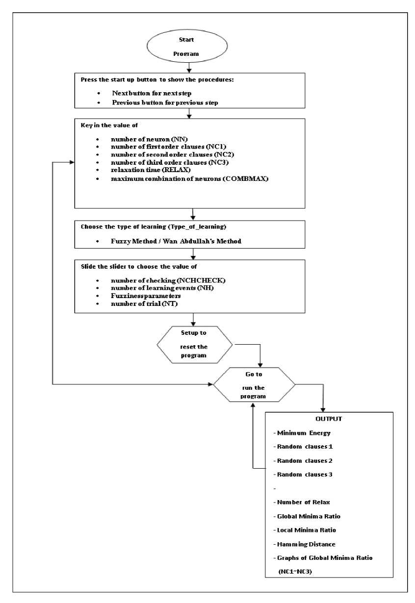
Fig.2 . Flow Chart for integrating fuzziness logic programming in the Hopfield neural network

Description of the flow chart [16]:

PHASE 1: Enter Values

• 1)    Press start-up / Reset Quick-Start button for a novel user.

• 2)    The user either presses the subsequent button so that he/she advances to the subsequent step or presses the preceding button so that the user retreats to the earlier step.

• 3)  Subsequently, the user can key in NN, NC1, NC2, RELAX, and COMBMAX.

• 4)    There is quite a small difference in higher orders as the NN maximum is 30. NC1, NC2, NC3 relate to the value of NN, which has been keyed in. The maximum RELAX and COMBMAX numbers are 100. The try and error technique has been used to select the entire values.

• 5)    Select the learning type that is the Hebb’s rule or Wan Abdullah’s approach.

• 6)  Next, the user slides the slider so that NCHCHECK, NH, TOL, as well as NT are selected.

• 7)  Maximum NCHCHECK, NH, as well as NT is 100, while the TOL value is selected as 0.5 after applying the

technique of trial and error.

• 8)    After setting the entire values, press the setup button for fixing and setting the program values.

• 9)    After that, the user presses the ‘go’ button to activate the program.

• 10)    It will produce random program clauses, e.g., when the user declares NC1 as 3, the 3 first-order clauses are created.

• PHASE 2: Training

  • 1)  The neurons’ initial states are set in clauses.

  • 2)    In accordance with the Hopfield network’s idea, which was originated from the behaviour of neurons (i.e., the particles) in a certain magnetic field, the particles are ‘communicating’ with each other and in a completely linked form with each particle striving to accomplish the energetically promising state, in other words, with a minimum of the energy function, called activation. All neurons in this state rotate to encourage each other to go on with rotation, allowing the network to evolve till minimum energy is reached. Consequently, the minimum energy corresponds to the wanted energy so that the global minima value is reached. Other programs that fuzzification integrated into Wan Abdullah’s method, are explained in section 4.

  • 3)    Testing of the final state (i.e., the accomplished state after the neurons’ relaxation). The final state is identified by the system as an unchanging state when it remains stable for 5 runs.

  • 4)    The stable state’s corresponding final energy can be calculated.

  • 5)    If there is a difference amongst the final energy, as well as the global minimum energy within the value of tolerance, the obtained solution will be global, or the user should return to step 1.

  • 6)    The user computes the global solution, along with the global solutions’ ratio (i.e., the ratio= Number of global solutions/ Number of iterations). Relaxation is run for 1000 trials; it is also run for 100 neurons’ combinations.

  • 7)    To conclude, the output of each run is printed out by the system.

6.    Simulations and Discussion

The cluster center is set, as well as the parameter of fuzzification v. = 4 and m = 2 . The technique of trial/error will generate all the values. No theoretical basis can be found to locate the most optimum choice of the parameter of fuzzification m . According to Bezdek [15], the algorithm is implemented for one of these values m >  1, which is selected as it can produce the ideal network performance. The pattern of training z is set to an initial state, including 1 or -1. The influence of ц is, thus, reliant on the value of m as the greater the m , the higher fuzziness value can be obtained.

The program has been operated for 100 trials, as well as 100 neurons’ combinations. The clauses number (NC) for every number of the neurons has been identified by the ratio between 0.1 and 1.0. A comparison is held for the global minima ratio (i.e., global solutions’ number/the runs’ number), in addition to the running time (that is, the needed time for the neurons’ relaxation toward final states) between direct method, as well as the FCM algorithm for logic programming to be performed in Hopfield network.

• A.    Hamming Distance

Hamming distance has been originally perceived for detecting and correcting errors [9, 19]. Simply, it is a differing bits’ number amid the two-bit vectors. Describing closeness of a certain bit pattern can be done easily to a differing bit pattern by determining the bit positions’ number, where both compared patterns differ. Therefore, the hamming distance has been measured between both states: the final state, as well as the global state.

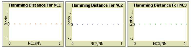
Fig.3. Hamming distances for NC1, NC2, and NC3

Fig. 3 displays the graphs of the hamming distance of each level of the clauses like NC1, NC2, and NC3. The Fig. 3 demonstrates that the hamming distance is almost close to zero, including all the cases if the neurons number (NN), with the number of the literals per clause (NC1, NC2, and NC3) amplified after applying the trial/error method. The hamming distance value is almost close to zero because neurons have reached a stable state. Therefore, the distance is approximately zero amid the given stable state, as well as the given global state. An identical statistical error is, therefore, obtained in the entire cases.

• B.    Global Minima

Based on the global minima graphs, when it is close to 1, it is assumed to approach the best solution [20].

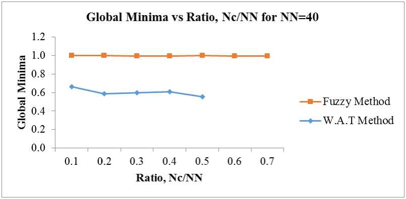
Fig.4. Global Minima for W.A.T method and fuzzy method, NN=40

Based on the conducted analysis, the achieved global minima ratio (i.e., the global minima values’ number/the number of the runs) of the FCM has been better compared to the direct method based on the figures above. The neurons have not yielded or trapped in any of the sub-optimal solutions. It can be observed that as the network’s complexity increased (i.e., the number of neurons grew larger), FCM performed more efficiently. This can be attributed to the modification and restriction of the cluster centers, as well as the energy function, thereby controlling the energy relaxation of every neuron. This, in turn, has enhanced the competence of controlling the energy relaxation process although the network has become larger. Therefore, the FCM method’s global minima ratio has outperformed compared to the given direct method. When the network can be complex, the direct method’s processing time has become bigger compared with FCM. The solutions also appear to oscillate; they are more easily stuck more with the given direct method.

• C.    Processing Time

Processing time is defined as a time acquired by a model to complete the training phase and retrieval phase[21].

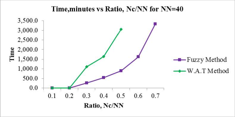
Time,minutes vs Ratio, Nc/NN for NN=40

3,500.0

3,000.0

2,500.0 " 2.000.0 P 1,500.0

1,000.0

500.0

0.0

0.1   0.2 0.3 0.4 0.5 0.6 0.7

Ratio, Nc/NN

—■—Fuzzy Method

—•—W.A.T Method

Fig.5. Processing Time for W.A.T method and fuzzy method, NN=40

As shown in Fig. 5, the technique of the fuzzy Hopfield neural network clustering can still maintain its consistency between 1.0 and 0.7 despite the increased network’s complexity. However, the values of global minimum solutions for the W.A.T method decreased up to 0.4. This proves that the technique of the fuzzy Hopfield neural network clustering is better than the W.A.T method. From Fig. 5, the processing time for the fuzzy Hopfield neural network clustering technique is better than the W.A.T method. Therefore, by utilizing the FCM method for enhancing the energy function, performing logic programming in the neural network can be enhanced.

7.    Conclusion

Agent-based modeling has been developed in this paper to perform logic programming in the Hopfield network by utilizing the NETLOGO platform. Based on the findings of the study, the FCM’s capability of performing logic programming on HNN has been more efficient compared to the method proposed by Wan Abdullah (only McCulloch pits updating rule applied to HNN). A better result has been provided regarding the global minima ratio and Hamming distance, as well as the CPU time. The results showed that FCMHNN enhanced the performing competence of logic programming if the neurons’ number is larger. Also, FCMHNN possesses a higher memory capacity; it did not undergo a substantial capacity loss if the input clauses are larger. Based on the experimental results, the introduced FCMHNN produced more promising results compared to HNN. Moreover, the designed FCMHNN represents a self-organized structure. It is enormously interconnected, used in an equivalent method, and easily designed for hardware gadgets to accomplish the high-speed application. However, finding the objective function’s global minimum by utilizing the Hopfield neural network remains a problem. Therefore, improving the FCMHNN training by using other algorithms such as ABC and AIS is recommended for further studies.

Acknowledgment

This research is supported by Research University Grant (RUI) (1001/PMATHS/8011131) by Universiti Sains Malaysia.