An Algorithm to Count Nodes in Wireless Networks Using their Actual Position

Published Online July 2016 in MECS

In the last few years, we have seen the growing and consolidation of two important technologies that are becoming ubiquitous. On one hand, wireless communication networks have revolutionized the way to send and receive information since they allow users’ mobility and lower the cost of network deployment. Nowadays, it is common to have access to communication networks from different devices such as smartphones, PDAs, tablets, notebooks, etc. On the other hand, the Global Positioning System (GPS) is a space-based satellite navigation system that provides location and time information, anywhere on the Earth where there is an unobstructed line of sight to four or more GPS satellites

• [1] . The GPS system is already heavily used in the automobile industry and it is becoming also very popular in smartphones.

The development of these technologies is promising and has attracted much interest from different entities that do research in these fields because of the multitude of possible applications that could involve their use. However, most of the possible applications require new algorithms and tools for their development. One such algorithm is the counting of objects (people, animals, devices, vehicles, etc.) with a specific characteristic or within a specified geographical area. Counting objects has interested the scientific community since time immemorial [2]. According to [3][4 ][5], there are many alternatives or solutions to count objects mainly based on “in situ” technologies, such as turnstiles, barrier arms, digital cameras, video cameras, thermal cameras, pneumatic road tubes, magnetic sensors, infrared beams, etc. However, since the installation and maintenance of these solutions are complex and have a high economic cost, it is necessary to propose alternatives. According to trends, in the near future, most of the mobile objects will be equipped of a wireless interface and a GPS receptor, hence a new possibility has been opened to develop counting algorithms based on these emerging technologies.

In this research work, we propose a novel algorithm to count nodes using wireless communications and their actual position. With the aim of validating the proposed algorithm, we use a discrete event simulator called OMNeT++/INET to test and analyze our proposal in different scenarios, where we varied different parameters such as nodes’ speed, nodes’ density, signal propagation range, etc. The simulation results show that our novel algorithm performs efficient node counting even when the nodes are moving at high speeds.

The rest of this paper is organized as follows. In Section II, we review the related work. In Section III, we introduce our novel algorithm to count nodes using wireless technologies and their actual position. Section IV briefly describes the simulation tools and scenarios that we use to validate the proposed algorithm. Section V presents an analysis of the performance results of our simulations. Finally, Section VI concludes the paper and presents future work.

• II.    Related Work

At the present time, most of the alternatives or solutions to detect and count nodes, with lesser or greater accuracy, are based on methods and techniques supported by conventional “in-situ” technologies (turnstiles, barrier arms, digital cameras, video cameras, thermal cameras, pneumatic road tubes, magnetic sensors, infrared beams, etc), which are used in many applications [6].

Many methods, techniques, and algorithms to count objects based on conventional “in-situ” technologies can be found in the literature. For example, there is a lot of work based in the usage of images or recordings of digital or video cameras. In [7], a face detection program is used to count people. Unfortunately, as pointed out by its authors, this method is affected by the angle of view at which the faces are exposed to the camera. Another approach has been suggested in [8] and aims to obtain an estimation of the number of people in the crowd, not the exact number of people. Bayona [9] proposed to perform a counting of people based on laser illumination and image processing techniques. In [10], the authors presented a method to count people who are in a subway station using video surveillance cameras. Kopaczewski et al. [11] introduced a method to estimate the number of people attending large public events, using the video signals gathered from multiple cameras and processing them with an efficient computer cluster. Knaian [12] developed a wireless sensor package to monitor roadways in the Intelligent Transportation Systems (ITSs) and count passing vehicles, as well as measure the average roadway speed, and detect ice and water on the road. Distributed people counting systems using wirelessly connected sensor nodes are discussed in [13][14 ][15][16]. The systems employ existing networking algorithms and protocols, available as part of the hardware platforms and operating systems used.

In the area of counting objects based on wireless technologies, very few works have been developed. For example, Gamess and Mahgoub [17] presented a novel VANET based approach to obtain: (1) the position of the last vehicle and (2) the number of vehicles, in a line of vehicles stopped at a traffic light. To compute the number of nodes, the authors first obtain the length of the queue of vehicles stopped at the traffic light and then divide this distance by a constant value (7 meters).

Unlike our proposal, as shown in this survey, most of the work done for counting objects is based on “in-situ” technologies.

• III.    Algorithm to Count Nodes Using Wireless Communications and their Actual Position

In this section, we describe our novel algorithm to count nodes based in their actual position using wireless technologies. To achieve the geographical location in this novel algorithm, each node is equipped with a Global Positioning System (GPS) receptor, allowing it to periodically send its actual position and speed through beacon messages.

• A.    Basic Considerations for Counting Nodes Using their Actual Position

The algorithm we present in this work represents an enhancement of the ideas raised in the work developed in [2]. As explained ahead, we added a neighbor discovery protocol and significantly improved the propagation of the COUNT_REPLY messages back to the originator.

To track the 1-hop neighbors, a neighbors discovery protocol was integrated to the nodes. Nodes periodically send BEACON messages with their actual position and speed, so that 1-hop neighbors are aware of their presence and position. Position and speed are obtained by nodes from their GPS receivers. Based on the received BEACON messages, a node establishes a list of 1-hop neighbors. For each 1-hop neighbor, the node stores its ID, timestamp, position, and speed. When receiving a new BEACON message from a 1-hop neighbor, the node updates its timestamp, position, and speed so that the last updated information is always present in the list of 1-hop neighbors. With this information, the node can interpolate the actual position of its 1-hop neighbors at any time. If a node does not receive three consecutive BEACON messages from a specific 1-hop neighbor (maybe because it has moved out of range), it removes this 1-hop neighbor from its list of 1-hop neighbors.

In this paper, we call “originator” the node that starts the counting process, i.e., the node that requires the number of nodes around it, up to a specified hop count (called HopLimit in the algorithm). Beside of the neighbor discovery protocol described before, the basic approach of the algorithm is:

• 1 . Propagate a broadcast message (called COUNT_REQUEST) from the originator to nodes that are far away from the originator with the number of HopAway the receiver of the message is from the originator of the COUNT_REQUEST.

• 2 .  Propagate unicast messages (COUNT_REPLY)

from the nodes that are far away from the originator toward the originator with the total number of nodes counted up to now (called Total in the algorithm).

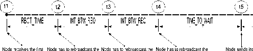
Fig. 1 depicts a timing diagram related to the propagation     of     the     broadcast     messages

(COUNT_REQUEST) and the unicast messages (COUNT_REPLY), where:

Node receives a

COUNT_REQUEST	COUNT_REQUEST	COUNT_REQUEST	COUNT_REQUEST	synchronous
	(1st rebroadcast)	(2nd rebroacast)	(3rd rebroadcast)	COUNT_REPLY

COUNT_REPLY COUNT_REPLY

Fig.1. Timing Diagram

Node sends an

delayed asynchronous

t1 = Time when a node receives the first COUNT_REQUEST t2 = t1 + RBCT_TIME t3 = t1 + RBCT_TIME + 1*INT_BTW_REQ t4 = t1 + RBCT_TIME + 2*INT_BTW_REQ t5 = t1 + REQ_TO t6 = Time when the actual node receives a possible delayed COUNT_REPLY message from another node.

t7 = Time when the actual node sends a possible asynchronous COUNT_REPLY message.

Fig. 1 also shows that the nodes will rebroadcast three COUNT_REQUEST messages in row and also send a synchronous COUNT_REPLY message after a specific time. It is necessary to send several times (3 times in our algorithm) the COUNT_REQUEST message since it is a broadcast message that can collide with other messages without this being detected.

In this new algorithm, each node sends its COUNT_REPLY message to another node, using the following considerations. If the nodeToGoBack is still on the list of 1-hop neighbors and if it is still in the node propagation range (according to the computation of the distance between the node and nodeToGoBack ), the node will send its COUNT_REPLY message to nodeToGoBack . Otherwise (when nodeToGoBack is out of range), the node determines the closest neighboring node toward the originator from its list of neighboring nodes (1-hop away nodes), by calculating the distance between the actual position of the 1-hop neighbor and the actual position of the originator, before sending the COUNT_REPLY message to this node. Additionally, the node updates its nodeToGoBack variable to point the calculated closest 1-hop neighbor. Now, if the node does not have any 1-hop neighbor in this moment (i.e., the list of 1-hop neighbors is empty), it will plan a new attempt to send its COUNT_REPLY message in the near future.

An asynchronous COUNT_REPLY message is sent by a node with a slight delay called DELAY_ASYNC, after receiving a delayed COUNT_REPLY message. This approach forces the cooperating nodes to update the actual node count, reaching a more accurate result.

The other parameters used in our algorithm are described here (see Fig. 1).

• •    INT_BTW_REQ (Interval Between Request): Time interval between the sending of COUNT_REQUEST messages. In other words, it also represents the time between two consecutive COUNT_REQUEST messages sent by the actual node.

• •    REQ_TO (Request Timeout): It is the time between the reception of the first COUNT_REQUEST and the moment when the actual node has to send the synchronous COUNT_REPLY message to nodeToGoBack toward the originator.

• •    TIME_TO_WAIT: It is the time a node waits after the rebroadcast of the third COUNT_REQUEST message and the sending of the synchronous COUNT_REPLY message to nodeToGoBack toward the originator. This time must be big enough to allow the propagation of COUNT_REQUEST messages from the actual node toward nodes that are far away from the originator, and the propagation of the COUNT_REPLY messages from the nodes that are far away from the originator toward the actual node. By the way, TIME_TO_WAIT is not a constant value and will be computed by every node according to HopLimit and how far away it is from the originator (called HopAway in the algorithm).

• •    DELAY_ASYNC: A small random time that a node waits after the reception of a delayed COUNT_REPLY message, and before the sending of the asynchronous COUNT_REPLY message.

• B.    COUNT_REQUEST and COUNT_REPLY Messages

COUNT_REQUEST and COUNT_REPLY messages have the same Protocol Data Unit (PDU) and are composed of 10 fields (see Fig. 2).

Message	Secuence Number	OrgTS	OrgX	OrgY	OrgSX	OrgSY	HopAway	HopLimit	Total
2 bytes	4 bytes	4 bytes	4 bytes	4 bytes	4 bytes	4 bytes	2 bytes	2 bytes	4 bytes

Fig.2. COUNT_REQUEST and COUNT_REPLY Messages

The field Message Type can be either 0 or 1. It is used to identify the type of message. A value of 0 is for a COUNT_REQUEST, while 1 is for a COUNT_REPLY. Sequence Number is used to match requests with replies and to distinguish between different requests (COUNT_REQUEST). OrgTS (Originator Timestamp) is set by the originator when it sends a COUNT_REQUEST message. It is a timestamp taken by the originator at the moment of sending the COUNT_REQUEST message and is aimed to control out-of-date messages and replay attacks. ( OrgX , OrgY ) is the position of the originator at the moment of sending the COUNT_REQUEST message. ( OrgSX , OrgSY ) is the speed of the originator at the moment of sending the COUNT_REQUEST message. The originator and the nodes broadcast COUNT_REQUEST messages along with the argument HopAway which represents the number of hops-away the receiver of the COUNT_REQUEST message is from the originator. The originator, which starts the process, must specify a value of HopAway equal to 1. Each node that rebroadcasts the message will select the smallest HopAway received up to now and will increment this field by 1. Every time a node updates its HopAway field due to the reception of a better COUNT_REQUEST (closer to the originator), it has to update its nodeToGoBack variable. nodeToGoBack is a reference to the node with the lowest HopAway from which the actual node has received a COUNT_REQUEST message. HopLimit field is a way to control how far away COUNT_REQUEST messages are propagated from the originator toward the other nodes. It delimits the counting range. The field Total is filled with the number of nodes counted up to now. In COUNT_REQUEST messages, it is always equal to 0. Before sending a COUNT_REPLY message, a node must update this field according to the COUNT_REPLY messages received so far, and add 1 to the sum that represents itself.

• C.    BEACON Messages

The PDU of BEACON messages are composed of 5 fields as shown in Fig. 3.

Timestamp         PosX           PosY         SpeedX         SpeedY neighboring nodes, the node chooses its new destination as the node that is currently closest (in distance) to the originator, using the information (Timestamp, PosX, PosY, SpeedX, SpeedY) gotten in the BEACON messages (see Fig. 3), and the information of the originator (OrgTS, OrgX, OrgY, OrgSX, OrgSY) received in the COUNT_REQUEST messages (see Fig. 2). This distance is computed applying the following formula:

distanceOrigin = path to the originator, as a unicast message. If after REQ_TO the node did not receive any COUNT_REPLY message, then it generates a COUNT_REPLY with Total equal to 1 (this 1 represents itself) and sends it to nodeToGoBack or the closest node in the path to the originator, as a unicast message.

• • DELAY_ASYNC: If the node receives a delayed COUNT_REPLY message, then it recalculates the total number of nodes based on variable Total received in the COUNT_REPLY messages (+1 to add itself to the total count) and then sends the result to its nodeToGoBack node or the closest node in the path to the originator, as an asynchronous COUNT_REPLY message.

• IV.    Environments and Scenarios of Simulation

The algorithm that we present in this paper was implemented in OMNeT++/INET. OMNeT++1 is an open source, C++ based, multiplatform (Windows, MacOS, and Unix), discrete event simulator for modeling any system composed of devices interacting with each other. One of the main strengths of OMNeT++ is its Graphical User Interface (GUI). Through the GUI, users can create NED files (a description language to define the structure of the model) and inspect the state of each component during simulations.

For simulations of data networks, OMNeT++ relies on external extensions, such as INET. The INET Framework is an open-source communication network simulation package for the OMNeT++ simulation environment. It contains models for several wired and wireless networking protocols, including UDP, TCP, SCTP, IP, IPv6, Ethernet, PPP, 802.11, MPLS, OSPF, and many others.

We chose OMNeT++/INET because of its powerful GUI that facilitates the traceability and debugging of simulation models, by displaying the network graphics, animating the message flow and letting users peek into objects and variables within the model. Also, it is a very active project with many models that are constantly updated, making OMNeT++ a good candidate for both research and educational purposes [18].

For all our simulations, we selected WiFi (IEEE 802.11g) for the wireless communication standard, with a bitrate of 54 Mbps. The free space propagation model was chosen for path loss. We simulate different scenarios where nodes are randomly distributed over a rectangular area. The random waypoint mobility model was selected to reflect the most general scenario of node movements.

• V.    Performance Results of our Simulations

In this section, we present and analyze some of the performance results of our simulations that were executed in scenarios with mobility: (1) in scenarios with mobile nodes and stationary originator and (2) in scenarios where both nodes and originator are mobile. We also execute simulations where we vary the size of the rectangular area where the nodes and the originator are placed and can move. We compare the results of our experiments with the ones obtained with the algorithm presented in [2].

• A.    Mobile Nodes and Stationary Originator Scenarios

In this section, we look at the performance of our algorithm when nodes are mobile, but the originator is static and placed in the center of an 800m x 800m squared area. For the movement of nodes, we use the random way point mobility model (RandomWPMobility) varying the speed of the nodes from 25 mps (meters per second) to 80 mps, with a wait time of 0s (time interval between reaching a target and moving toward the new one).

In Table 1, we varied the propagation range of the nodes and the originator (100m, 150m, 200m, 250m, and 300m). For all these scenarios, we chose 100 mobile nodes that are initially randomly placed with value of RBCT_TIME=0.2s, INT_BTW_REQ=0.2s, and DELAY=0.4s. The originator starts the counting process with hopLimit =3.

The results are represented as values a / b/c , where a denotes the number of nodes that are within the scope of the originator using multihop routing (i.e., nodes that should be counted), b the number of nodes actually counted by the algorithm of [2] (that from now on we will call Algorithm I ), and c the number of nodes actually counted by our novel algorithm (which we will call hereinafter Algorithm II ). According to these results, we can observer that we have high accuracy in the nodes counting with algorithm II . We can see that the best results are obtained with values of propagation range equal to 200m, 250m, and 300m. For example, Table 1 shows that for a scenario of 100 nodes, a propagation range equal to 200m, and a speed equal to 55 mps (198 km/h), the originator should count 100 nodes. Now when we run the simulation, algorithm I counted 50 nodes, instead of 100 nodes, which is a good approximation. However, algorithm II counted 90 nodes, being much more effective.

In Table 2, we chose a fixed propagation range of 250m, but we varied the speed of the nodes (from 25 mps to 80 mps) and the number of nodes. Based on these results, we can see that for a number of nodes up to 100, algorithm II performs an effective counting even for very high speeds compared with algorithm I. Now, in both algorithms when there is a high density of nodes (when the total number of nodes is equal to 150, 200, and 250), the accuracy of the counting degrades. This is due to the numerous collisions, since there are many nodes in a small area trying to send messages at the same time. It is worth mentioning that algorithm II is still performing a more effective counting than the other one, even in these adverse conditions.

• B.    Mobile Nodes and Originator Scenarios

In this section, we report results of experiments when both the nodes and the originator are mobile. At the beginning of the simulations, the nodes are randomly positioned in an 800m x 800m squared area, while the originator is initially placed at its center. Both, the nodes and the originator are moving according to the random way point mobility model, without making stops at the visited positions, i.e., with a wait time of 0s. For both, nodes and the originator, we chose RBCT_TIME=0.2s, INT_BTW_REQ=0.2s, and DELAY=0.4s. The originator starts the counting process with a hopLimit=3.

Table 1. Nodes Counted when Varying the Speed of the Nodes and the Propagation Range (Speed Originator = 0 mps)

Nodes speed (mps)	Propagation range values in meters
	100m	150m	200m	250m	300m
25	38/12/34	96/35/88	100/50/92	100/71/98	100/73/97
30	30/15/29	93/38/85	100/55/96	100/64/100	100/75/93
35	46/19/43	87/37/78	98/52/81	100/72/93	100/74/90
40	53/5/44	87/32/84	100/63/99	100/56/91	100/75/99
45	44/11/33	92/29/83	100/31/81	100/44/95	100/60/90
50	49/12/38	95/27/90	100/37/76	100/53/96	100/62/98
55	47/16/30	87/21/79	100/50/90	100/68/99	100/72/94
60	51/6/49	93/28/84	99/49/82	100/64/90	100/70/100
65	58/6/50	93/9/67	100/33/85	100/63/97	100/66/91
70	48/5/48	91/11/86	100/29/97	100/39/93	100/56/94
75	35/1/35	85/23/81	100/29/83	100/45/91	100/51/93
80	43/7/42	87/16/65	100/25/84	100/44/90	100/54/91

Table 2. Nodes Counted when Varying the Speed of the Nodes and the Number of Nodes (Speed Originator = 0 mps)

Nodes speed (mps)	Total number of nodes
	60	70	80	90	100	150	200	250
25	60/46/60	70/52/62	80/58/77	90/76/90	100/71/91	150/90/142	200/124/184	250/112/221
30	60/46/59	70/47/69	80/59/74	90/62/84	100/64/96	150/78/141	200/109/193	250/129/213
35	60/39/59	70/49/68	80/51/77	90/64/84	100/72/92	150/89/141	200/112/179	250/123/214
40	60/39/58	70/50/68	80/49/77	90/65/85	100/56/99	150/90/138	200/106/153	250/133/233
45	60/32/57	70/48/61	80/59/71	90/67/85	100/44/99	150/88/138	200/129/181	250/128/213
50	60/38/60	70/39/64	80/51/77	90/71/88	100/53/95	150/82/123	200/107/185	250/120/224
55	60/30/60	70/37/65	80/54/80	90/61/84	100/68/100	150/91/126	200/118/140	250/134/197
60	60/28/58	70/40/65	80/61/72	90/57/89	100/64/98	150/64/133	200/127/176	250/115/207
65	60/40/59	70/36/62	80/52/73	90/53/87	100/63/94	150/64/133	200/108/176	250/110/200
70	60/41/56	70/46/69	80/35/79	90/47/90	100/39/96	150/57/136	200/94/182	250/91/202
75	60/30/58	70/38/67	80/34/77	90/41/88	100/45/91	150/68/134	200/95/144	250/89/185
80	60/33/58	70/28/70	80/32/73	90/48/83	100/44/99	150/68/128	200/76/177	250/87/188

Table 3. Nodes Counted when Varying the Speed of the Nodes and the Originator as well as the Number of Nodes

Speed (mps)	Total Number of Nodes
	60	70	80	90	100	150	200	250
25	60/50/60	70/43/69	80/61/79	90/45/90	100/57/91	150/61/122	200/103/113	250/154/216
30	60/50/58	70/49/68	80/59/78	90/45/84	100/42/96	150/73/138	200/82/114	250/153/223
35	60/40/60	70/42/66	80/31/75	90/34/84	100/65/92	150/36/134	200/60/186	250/140/214
40	60/44/54	70/50/68	80/26/79	90/32/85	100/68/99	150/84/132	200/73/173	250/129/208
45	60/39/58	70/47/68	80/52/77	90/45/85	100/66/99	150/75/138	200/93/126	250/71/204
50	60/33/60	70/42/67	80/29/76	90/16/88	100/43/95	150/64/133	200/92/166	250/92/181
55	60/19/57	70/22/69	80/45/74	90/60/84	100/56/100	150/67/130	200/64/176	250/51/202
60	60/27/60	70/31/63	80/55/79	90/45/89	100/64/98	150/69/125	200/78/173	250/89/216
65	60/35/53	70/49/70	80/44/77	90/29/87	100/70/94	150/46/126	200/72/166	250/91/205
70	60/29/56	70/46/68	80/45/76	90/27/90	100/41/96	150/72/127	200/36/161	250/102/212
75	60/18/60	70/21/70	80/19/77	90/26/88	100/45/91	150/50/119	200/78/160	250/69/198
80	60/14/57	70/21/69	80/18/77	90/41/83	100/34/99	150/83/115	200/63/155	250/85/193

Table 4. Nodes Counted when Varying the Speed of Nodes and the Originator as well as the Propagation Range

Speed (mps)	Propagation range values in meters
	100m	150m	200m	250m	300m
25	6/3/5	23/15/22	64/30/55	100/57/91	100/75/98
30	10/6/10	38/14/33	57/32/57	100/42/96	100/57/98
35	21/6/19	49/11/48	78/27/78	100/73/92	100/84/97
40	28/13/19	58/21/56	83/58/78	100/63/99	100/80/97
45	35/10/25	73/16/58	94/60/82	100/47/99	100/74/99
50	43/6/17	86/14/70	100/55/90	100/44/95	100/76/95
55	47/4/29	89/13/52	100/37/83	100/20/96	100/56/97
60	31/3/30	89/23/77	100/25/86	100/49/98	100/41/98
65	21/4/12	76/16/51	94/38/80	100/46/94	100/50/94
70	16/4/14	48/10/37	90/43/88	100/56/96	100/69/96
75	14/3/13	38/7/27	81/24/81	100/40/91	100/65/91
80	19/2/10	62/5/61	88/26/83	100/31/99	100/45/99

In Table 3, we chose a fixed propagation range of 250m, but we varied the speed of the nodes and the originator (from 25 mps to 80 mps), as well as the number of nodes. As in the experiments of Table 2, the novel algorithm performs a most effective counting than algorithm I for a number of nodes up to 100. Now, for high density of nodes, in both algorithms the accuracy of the counting degrades due to the numerous collisions, but being significantly more efficient in algorithm II.

Table 4 shows the results of the simulations for scenarios with 100 nodes, where we varied the speed of the nodes and the originator, as well as their propagation range. Similarly to Table 1, we can see that algorithm II has a higher precision in the counting of nodes than algorithm I , specifically when the propagation range values are equal to 200m, 250m, and 300m.

• C.    Other Simulations

In this section, we study the performance of the proposed algorithm on the perspective of the response time and the number of messages sent by the nodes, in scenarios where both the nodes and the originator are mobile. At the beginning of the simulations, the nodes are randomly positioned in an 800m x 800m squared area, while the originator is initially placed at its center.

Table 5 shows the results of the experiments for scenarios where we varied the total number of nodes (from 60 to 250) and chose a fixed propagation range value of 250m and a speed of the nodes and the originator equal to 55 mps (198 km/h). We can observe that algorithm II performs an effective counting for a number of nodes up to 100 with a small number of messages and a short response time. For example, for a total of 100 nodes, 98 out of 100 reachable nodes were counted effectively by our novel algorithm in 3.17s, with a total number of sent messages equal to 519 and a counting error of 2%.

In Table 6, we varied the speed of the nodes and the originator (from 25 mps to 80 mps). For all these scenarios, we chose 150 mobile nodes and a fixed propagation range value of 250m. Similarly to Table 5 the simulation results show good response times with a small number of messages. For example, as reported in Table 6, for a speed of nodes and the originator equal to 65 mps (234 km/h), a total number of nodes equal to 150, and a propagation range of 250m, 144 out of 150 reachable nodes were counted by our novel algorithm in 3.07s, with a total number of sent messages (COUNT_REQUEST and COUNT_REPLY) equal to 896 and a counting error of 4%.

We also performed some experiments by changing the size of the rectangular area with a density of 100 nodes/km² (see Table 7) with the aim of evaluating how the size of the area can affect the algorithm, and thus check if it presents scalability issues. At the beginning of the simulations, the nodes are randomly positioned in a rectangular area, while the originator is placed at its center. Both, the nodes and the originator are moving according to the random way point mobility model, without making stops at the visited positions, i.e., with a wait time of 0s and a speed of 55 mps (198 km/h). For both, nodes and the originator, we chose RBCT_TIME=0.2s, INT_BTW_REQ=0.2s, and DELAY=0.4s and a fixed propagation range of 250m. The originator starts the counting process with a hopLimit =3. In general terms, simulation results show that our algorithm also performed well, in different sized areas, at high speeds, with a small number of messages and an acceptable response time.

Table 5. Response Time and Number of Sent Messages when Varying the Number of Nodes

Total number of nodes	Propagation range value = 250m
	Reachable nodes	Nodes count algorithm	Response time	Counting error	Total messages sent
60	60	52	3.18s	13.3%	286
70	70	64	2.94s	8.6%	295
80	80	75	2.84s	6.3%	365
90	90	86	3.10s	4.4%	477
100	100	98	3.17s	2.0%	519
150	150	137	3.27s	8.7%	823
200	200	177	3.39s	11.5%	989
250	250	215	3.49s	14.0%	1279

Table 6. Response Time and Number of Sent Messages when Varying the Speed of Nodes and the Originator

Speed (mps)	Total number of nodes = 150 and propagation range = 250m
	Reachable nodes	Nodes count algorithm	Response time	Counting error	Total messages sent
25	150	143	3.27s	4.7%	806
30	150	145	3.00s	3.3%	692
35	150	138	3.20s	8.0%	803
40	150	141	3.78s	6.0%	953
45	149	144	3.45s	3.4%	792
50	150	146	3.35s	2.7%	714
55	150	137	3.27s	8.7%	823
60	150	130	2.90s	13.3%	636
65	150	144	3.07s	4.0%	896
70	150	129	3.61s	14.0%	678
75	150	136	3.57s	9.3%	766
80	150	131	3.08s	12.6%	742

Table 7. Nodes Counted when Varying the Size of the Rectangular Area (Mobil Nodes and Originator)

Size of the area	Total number of nodes	Reachable nodes	Nodes count algorithm	Response time	Counting error	Total messages sent
500m x 500m	25	25	20	2.04 s	20.0%	128
500m x 750m	38	38	38	2.96 s	0.0%	161
500m x 1000m	50	50	50	4.91 s	0.0%	495
500m x 1250m	63	63	58	3.18 s	7.9%	529
500m x 1500m	75	71	64	3.65 s	9.9%	639
750m x 800m	60	60	59	3.26 s	1.7%	414
750m x 1000m	75	64	64	5.78 s	0.0%	441
750m x 1250m	94	89	70	3.55 s	21.3%	614
800m x 800m	64	64	59	2.83 s	7.8%	276
800m x 1000m	80	80	73	2.85 s	8.8%	355
800m x 1250m	100	97	83	3.06 s	14.4%	607
1000m x 1000m	100	100	90	2.72 s	10.0%	399
1000m x 1250m	125	109	99	3.65 s	9.2%	936
1250m x 1250m	156	141	124	2.84 s	12.1%	671
1500m x 1500m	225	182	162	4.19 s	11.0%	1238
2000m x 2000m	400	197	178	5.14 s	9.6%	1279

• VI. Conclusions and Future Work

In this paper, we described a novel algorithm to count nodes using wireless communication and their actual position, based on the ideas raised by the algorithms proposed in [2]. The new algorithm differs from the previous one with the addition of position and speed information, to make wiser decisions when sending COUNT_REPLY messages back to the originator. For that, a discovery protocol was implemented where BEACON messages are sent periodically, allowing nodes to discover their 1-hop neighbors and infer their actual position at any time. Another enhancement of the algorithm is the introduction of late COUNT_REPLY messages, in order to recalculate the total number of nodes, and obtain a better counting.

To validate and evaluate the performance of our novel algorithm, we performed simulations where fast mobility is involved in the experiments, resulting in frequent topological changes between devices, specifically: (1) in scenarios with mobile nodes and stationary originator and (2) in scenarios where both nodes and the originator are mobile. We compare our new algorithm with an algorithm proposed in [2]. Simulation results indicate that our novel algorithm efficiently computes a total number of nodes very close to the real one, even in scenarios when the nodes are moving at very high speed, with a small number of messages and a short response time. However, for scenarios with a high density of nodes, the accuracy of the counting degrades for both algorithms, due to the great amount of collisions that occur in the sending of messages, but still significantly more efficient in the algorithm proposed in this investigation.

Moreover, we also performed some experiments where we varied the size of the rectangular area where nodes and the originator are placed and moved, with the aim of evaluating how the size of the area can affect the algorithm, and test it for scalability issues. In this case also, simulation results show that our new algorithm also performs a more efficient counting, in different sized areas, at high speeds.

As possible future work, we plan to adapt our algorithm to wireless networks with multichannels with the intention of reducing the collisions that occur between the counting PDUs (BEACON, COUNT_REQUEST, and COUNT_REPLY) and users’ traffic, and thus, possibly improve the accuracy of the counting in scenarios with high density of nodes. We are also interested in studying the application of our algorithm in the vehicular context (motorways, urban roads, rural roads, parkings, etc) using Wireless Access in Vehicular Environment (WAVE) [19], which could be used in applications to improve the safety and comfort of drivers and passengers.

Acknowledgment

We thank the CDCH-UCV (Consejo de Desarrollo Científico y Humanístico) which partially supported this research under grant number: PG 03-8066-2011/1.