An Approach of Degree Constraint MST Algorithm

Combinatorial algorithms concern the problems of performing computations on discrete, finite mathematical structures. The subject of combinatorial algorithms often referred as combinatorial computing, deals with the problem of computing discrete mathematical structures. It is a new field derived from systematic body of knowledge about the design, implementation, and analysis of algorithms appeared from a collection of tricks distinct algorithms. Combinatorial computing has an important role for representation and solving the graph theory problems like generation of all trees and cliques etc.

Graph theory algorithm can be trace back over one hundred years to when Fleury gave a symmetric method for tracing an Eulerian graph and G. Tarry showed how to escape from a maze. During the 20th century such algorithms increasingly came into their own, with the solution of such problems as the shortest and longest path problems, the minimum connector problem, and the Chinese postman problem. In each of these problems we are given a network, or weighted graph, to each edge of which has been assigned a number, such as its length or the time taken to traverse it.

Graph theory, an important branch of engineering has wide applications in the fields of chemistry, computer science, mobile computing, networking, social science, cryptography and many more. Generation of all trees of a graph is even fabulous and it is a kind of NP-complete problem. Solving this type of problem we generally use some heuristics approach and it has application in topology design and networking. Lists of some NP-complete problems are given in the section 4 in this paper. There are several algorithms to generate minimal spanning tree of a weighted graph like Kruskal, Prim algorithms and some new algorithms also discovered which is optimal in respect of execution time comparing to the existing one.

Graph theory finds wide influence in computer science and mathematics. Graphs, especially trees and binary trees are widely used in the representation of data structure [1, 2, 3, 4].

A Tree is a connected linear graph without any circuit. The concept of a tree is the most important in the graph theory, especially for those interested in applications of graphs. A linear graph G=(V, E) consists of a set of objects V={v 1 , v 2 , v 3 ,…..} called vertices, and another set E={e 1 , e 2 , e 3 ,……} called edges, such that each edge e k is identified with an unordered pair (v i , v j ) of vertices. A tree is nothing but a simple graph that is, having neither a self-loop nor parallel edges. Tree appears in numerous instances. The genealogy of a family is often represented by means of a tree. In facts the term tree comes from family tree. In many sorting problems we have only two alternatives at each intermediate vertex, representing a dichotomy, such as large or small, good or bad, 0 or 1. Such a decision tree with two choices at each vertex occurs frequently in computer programming and switching theory.

The concept of tree appeared implicitly in the work of Gustav Kirchhoff (1824 - 1887), who employed graph theoretical ideas in the calculations of currents in the electrical networks or circuits. The enumeration techniques involving trees first arose in connection with a problem in the differential calculus, but they soon came to the fundamental tools in the counting of chemical molecules, as well as providing a fascinating topic of interest in their own right. Cayley was led by the study of the particular analytical forms arising form differential calculus to study a particular types of graphs, the ‘tree’. This study has many implications in theoretical chemistry. This involved techniques mainly concerned the enumeration of graphs having particular properties. Arthur Cayley (1821 - 1895), James J.

Sylvester (1806 - 1897), George Polya (1887 - 1995), and other use tree to enumerate chemical molecules. Recently, a wide variety of new results in combinatorial enumeration have been obtained. Many of these results were promted by new problems in computer science, while others answered old questions in combinatorics and other fields. The aim is to survey on history of tree and a subset of the new results, namely those dealing with tree enumeration.

A Spanning Tree is a tree of a connected graph G, which connect all vertices of the graph. If G is a connected graph of n vertices, the spanning trees are the subsets of n-1 edges that contain no cycles; equivalently they are subsets of edges that form a free tree connecting all the vertices. Spanning trees are important in many applications, especially in the study of networks, so the problem of generating all spanning trees has been treated by many authors. In fact, systematic ways to list them all were developed early in the 20th century by Wilhelm Feussner (Annalen der Physik, 4, 1902, 1304 - 1329), long before anybody thought about generating other kinds of trees. Generation of a single spanning tree for a simple, symmetric and connected graph G, is a classical, and one polynomial time solvable problem [5, 6].

The goal of optimization of minimal spanning tree is to find an appropriate solution [1, 7]. When studying diverse problems, one often makes an assumption of general position: for minimal spanning trees, one can infinitesimally perturb the distinct edge weights in this way to choose out a unique solution. Several algorithms exist for generation of Minimal Spanning Tree [8]. In Otakar Boruvka’s algorithm of finding a Minimal Spanning Tree in a graph, all the edge weights are distinct. In 1957, Computer Scientist C. Prim discovered another algorithm that finds a minimal spanning tree for a connected weighted graph [8]. This algorithm continuously increases the size of a tree starting with a single vertex until it spans over all the vertices. This algorithm was actually discovered in 1930 by mathematician Vojtech Jarnik. Similarly Joseph Kruskal and Edsger Dijkstra in 1959 have given different algorithms about finding minimal spanning tree. In 1981 coauthor Samar Sen Sarma introduced an algorithm in his paper for generation of all spanning trees of a simple connected graph. There is no possibility of duplicity if the spanning tree is generated by this algorithm, and also prohibits generation of all the non-tree sub-graphs.

Again in 2007, authors have discussed an algorithm where trees are generated by probing eC sets of edges where e is the number of edges and n is the number of vertices of a simple connected graph eliminating some set of edges which form circuit [9]. This paper reveals a new algorithm for creating minimal weight spanning tree of a graph which requires less execution time and memory space compared to the existing algorithm. The algorithm is based on the degree factor of the degree sequence and the weight of edges in the graph G. A sequence d , d , d , d ,...., d of nonnegative integers is called a degree sequence of given graph G, if the vertices of G can be labeled Vj, V2, V3, V4,..., Vn so that degree v; = d;; for all

• i.    The sum of the integers d , d , d , d , , d is equal to 2e, where e is the number of edges in a graph G [10]. For a given graph G, a degree sequence of G can be easily calculated. Now the problem arises that, given a sequence ^ = d_Y , d^ , d₃ , d₄,...., d_n of nonnegative integers, under what conditions does there exist a graph G? An essential and adequate condition for a sequence to be graphical was found by Havel and later rediscovered by Hakimi. Based on the above views we commence a new method to find out a minimal spanning tree of a graph G considering degree sequence factor of the nodes as constraint. The time complexity and space complexity of the new algorithm are optimal in comparison to the algorithms of Kruskal and Prim.

In section 2, of the paper covers some basic terminology used in the paper. The basic technique used to generate the MST algorithm has been described in section 3. It has been followed by some theorems as foundation of the logic development and understanding of the paper. Section 4, describes the algorithms of degree constraint MST (main theme of this paper) and section 5, describes circuit testing algorithm which is used to implement the main algorithm. The complexity of the new algorithm has been described in section 6. In section 7, we have presented execution time of Kruskal, Prim, and new algorithms as part of the comparative study and analysis of execution time between algorithms. Finally, references have been given at the end of the paper which has helped us to get a direction.

• II.    Terminology

• 2.1    Graph

In this section basic terminology has been given which is used in the next part of this paper.

An undirected, simple, connected graph G is an ordered triple (V(G), E(G ), f) consist of

• •    a non empty set of vertices n £ V of the graph G

• •    a set of edges e e E of graph G and

• •    a mapping f from the set of edges E to a set of unordered pair of elements of V.

• 2.2    Tree:

• 2.3    Spanning Tree

• 2.4    Minimal Spanning Tree

A tree T of a graph G is a simple, connected and acyclic graph having exactly one path between the vertices so that we can traverse any vertex to any others vertices along the edges. In other words, a tree is a simple connected graph without any self-loops or parallel edges.

A Spanning Tree S is a tree of a connected graph G, which touches all vertices of the graph. A spanning tree has n vertices and exactly (n-1) edges of a graph G.

Let G be a connected, edge-weighted graph. A minimal spanning tree is a subgraph of G that satisfies the following properties:

• •    It is a tree , that is, it is connected and has no cycles.

• •    It is spanning , that is, it contains all vertices of G .

• •    It has minimal total edge-weight among all possible trees.

• 2.8    Average Degree

Node Degree FactorSum of Degree of all nodes deg ree of a node

n

E di i=1 d(ni)

It is the ratio between summations of degree of all nodes of the graph G to number of nodes i.e.

A var age Degree ( v J

Summetion of Degree of nodes of graph Total number nodes

n

E di

_ i=1 n

• 2.9    Realization

• 2.5    Adjacency Matrix

• 2.6    Degree of a Vertex

• 2.7    Node Degree Factor

A sequence £ = dx, d2, d3, d4,...., dn    of nonnegative integers is said to be graphic sequence if there exists a graph G whose vertices have degree d and G is called realization of ξ.

For a graph G of n vertices and e edges, if, set of vertices, V(G) = {v 1 , v 2 , v 3 ,……, v n } and set of edges E(G) = {e₁, e₂, e₃,……, e_n}. The adjacency matrix A, of weighted graph G, is n x n matrix and it can be represent by A = [a ij ], where

I w„ if there is an edge between v , v . e E ( G ) a = s ^{J                                     J}

‘j   [0 if there is no edge

The degree d i of a vertex v i in a graph G is the number of edges connected with v_i. In other words, degree d_i is the number of vertices adjacent to the vertex v i .

It is the ratio between summations of degree of nodes of graph G to degree of a node / vertex i.e.

• III.    Minimal Spanning Tree Generation

A tree having n nodes and n-1 edges is spanning tree of a graph. A preferable and efficient algorithm is one that generates trees by selecting only the minimal cost edges of the graph and also by not producing cycle. The present algorithm is still required to test circuits for some cases. This new algorithm is more efficient in terms of the required execution time. In this algorithm, first we calculate average degree of each node and then identify a node v k having degree is equal to average degree v a or more in the graph. This will identify a node in the graph G and an edge having minimum weight edge incident on it. This minimum weight edge incident to vertex v_k,is to be included in the list of constructing minimal spanning tree (S), if the edge does not form circuit in S and not selected previously.

• Theorem 1:    A spanning tree S of a weighted connected graph G is the minimal weight spanning tree if and only if there exist no other spanning tree of G at a distance of one from S whose weight is smaller than that of S.

Proof: Let S1 be a spanning tree in graph G satisfying the hypothesis of the theorem there is no spanning tree at a distance of one (of G) from S1 which is smaller than S1. If S2 is a smallest spanning tree in G, the weight of S1 will also be is equal to that of S2. The spanning tree S2 is smallest if and only if, it satisfies the hypothesis of the theorem.

Suppose, an edge e in S2 is selected based on the least weight of the vertex of the graph G but it is not in S1. Adding e to S1 forms a fundamental circuit with branches of S1. Some of the branches in S1 that form fundamental circuit with e in S2; each of the branches of S1 has weight either smaller than or equal to e because S1 is minimal weight. Amongst all these edges of circuit but not in S2, at least one, say b, must form fundamental circuit in S2 containing e. So, b must have same weight as e. Therefore, spanning tree 5[ = ( 5 ^ О ( e — b )) , obtained from S1, though one cycle exchange, has sane weight as S1. S1 has one more edge common with S2 and it satisfies the condition of theorem.

• Theorem 2:    An edge e corresponding to the vertex of minimal weight in the graph G is form a spanning tree, if it has minimal weight.

Proof: A spanning tree S of a graph G contains all the vertices (exactly once) and n-1 edges, where n is the number of vertices. An edge e to be selected based on the weight of the vertex. The weight of a node shows the average weight of the edges incident to it. The minimal weight of the vertex indicates that there must have at least one edge whose weight is minimal and it could include in the spanning tree S, if and only if, at least one end vertex is not yet colored (included in S). To avoid the generation of fundamental circuit in the minimal spanning tree S, we select only those edges whose, at least one vertex is not yet colored. If edge e form fundamental circuit in minimal spanning tree S then we will select another edge corresponding to the same vertex whose weight is either equal to or just higher than edge e.

• Theorem 3:    The combination of n-1 distinct edges is formed spanning tree according to theorem 1, if it is circuit less.

Proof: The n-1 edges combinations of a graph must contain all the vertices of the graph. This combination either contains a circuit or a spanning tree of the graph. Thus to ascertain its calm as spanning tree circuit testing is necessary.

• Theorem 4:    An edge e corresponding to the node of highest degree factor in the graph G forms a spanning tree, if it has minimal weight.

Proof: A spanning tree S of a graph G contains all the vertices (exactly once) and n-1 edges, where n is the number of vertices. An edge e is to be selected based on the degree factor of the node. The degree factor of the node shows how many edges are incident to a particular node. The highest degree factor of a node, the number of edges incident to which is minimum with at least one edge whose weight is minimal, is to be included in the minimum spanning tree S.

• Theorem 5:             A            Sequence

D = d. , d ₂, d ₃, d ₄,...., d„ of nonnegative integers with d_Y >  d^ >  d ₃ >  d₄ .... >  d_n , n > 2, d_Y >  1 is graphical if and only if the sequence D = d 2 - 1, d 3 - 1, d 4 - 1,...., d d + 1 - 1, d d _{+ 2},....,d n is graphical [11].

Proof: Let D' is a graphical sequence. There exists a graph G of order n-1, such that D' is the degree sequence of G . Therefore, the vertices of G can be labeled as V2, V3,.., Vn ; such that deg( V) =

dY — 1; 2 < i < dY +1 dY; dY + 2 < i < 1

A new graph G can be constructed by adding a new vertex V and the d_Y edges VV ; 2 <  i <  d_Y + 1 . Then in G , deg(V_i) = d_; for 1 <  i <  n and so D = dj, d₂, d₃, d₄, ^ ,d_n is graphical.

Conversely, let D be a graphical sequence. Hence there exist graphs of order n with degree sequence D. Among all such graphs let G be one, such that        V(G) = { V ₁ ,V ₂ ,V 3 ,V ₄ , _ ,V _n }        ;

degCV) = d; fori = 1,2,3,,...,n and the ^d; = even number, the sum of degrees of the vertices adjacent with V is maximum. we show first that V is       adjacent       to       vertices       having degreesd2, d3, d4,.,ddi+1.

suppose, to the contrary, that V is not adjacent to vertices having degrees d2, d3, d4,.,dd +1 . Then there exist vertices V and V with dr > ds such that V is adjacent to V , but not to V . since, the degree of V exceeds that V , there exists a vertex V , such that V is adjacent to V but not to V . Removing the degrees V V and V V and adding the edges V V and V V results in a graph G having the same degree sequence as G. However, in G the sum of the degrees of the vertices adjacent to V is larger than that in G, contradicting the choice of G. thus, V is adjacent with vertices having degrees d , d , d ,…,d , and the graph (G -V ) has degree sequence D ′ , so D ′ is graphical.

Theorem 6: If a subgraph of n-1 edges contains more than three nodes of degree more than one and if there is no pendent edge in the graph, the subgraph contains a circuit.

Proof: For simplicity and to explain the theorem easily, we take into consideration a simple connected graph as shown in the figure given below.

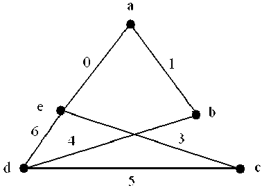
Fig. 1: A Simple Connected undirected Graph

In the above combination, there are two vertices of degree one and three vertices of degree more than one, hence this combination may give the circuit. Deleting pendent edges incidence on vertex a and b, the modified degree of all the vertices are,

Node No:    a  b  c  d  e

Degree:     0  0  2   2  2

Since, the degree of all the three vertices are more than one, this is confirmed that the edge combination will produce a circuit. The pictorial form of this combination is shown in figure 3.

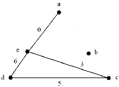
Fig 3: An Illustrative Circuit of Graph shown in Fig. 1

From the given graph in figure 1, if we consider the edge combination, 1 4 5 6 2, the degree of each vertices corresponding to the given edge combination are,

Node No: a b c d e

Degree: 13 13 1

Since there are three vertices of degree one and only two vertices of degree more than one, hence this n-1 edges combination will not produce a tree of the graph G. The pictorial form of this tree is shown in the figure given below.

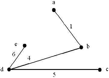
Fig 2: An Illustrative Tree of Graph shown in fig.1

Considering another example, if edge combination is, 0 3 5 6 2, of the graph shown in figure 1, the degree of each vertices corresponding to the given edges combination are,

Node No:    a b c  d  c

Degree:    112  2 3

• IV.    Algorithm of Constraints based Minimal Spanning Tree Generation

Initially we generate random weighted graph according to the given number of nodes and edge density. The weight matrix of the randomly generated graph is used as input for generation of minimal spanning tree of the graph. The output of the algorithm is minimal weight spanning tree (S) where each node of the graph is represented by the edge number from 0,1,2,……..,n. The weight, w of the edge is stored in the adjacency matrix if there is an edge between the nodes.

Step 4.1: Generate random weighted graph and corresponding weight matrix according to the given number of nodes and edge density.

Step 4.2: Calculate average degree (v_a) of nodes using the formula shown in section 2.8. Since average degree of node is v a therefore, maximum degree of a node in constructing minimal spanning tree will be consider is lower value of v a i.e. [Vq- .

Step 4.3: Select any node v_k having average degree v_a or more in graph G, for construction of minimal spanning tree.

Step 4.4: Select a minimum weight edge e which is adjacent to node v k , put this edge into constructing MST, so that the edge do not form circuit and degree of v_k could not be more than average degree v a .

Step 4.5: Construct new graph G ′ removing the edge already selected in constructing minimal spanning tree and assign G ′ into G.

Step 4.6: Apply iteratively step 3 to step 5, till (n-1) edges are not selected into constructing Minimal Spanning Tree.

Step 4.7: Calculate sum of the weight of the edges in the constructing MST, S.

Step 4.8: Display/store output.

Step 4.9: Stop.

• V.    Circuits Testing Algorithm

The circuit testing algorithm is used to find out the circuit in the constructing spanning tree is given below.

Step 5.1: From n-1 edges and incidence matrix degree of each node is obtained which is contributed by n-1 edges under consideration.

Step 5.2: Testing is done whether at least two nodes of degree one exits or not. If not, step 6 is executed. Otherwise the process is continued.

Step 5.3: It is tested whether at least three nodes of degree or more than one is present or not. If not, then step 5 is followed.

Step 5.4: Pendant edges are deleted, if there is existence of n-1 edges and the degree of the nodes are modified accordingly and is carried on to step 2. Otherwise step 6 is executed.

Step 5.5: Edge combinations are tree.

Step 5.6: Stop.

• VI.    Complexity of the Algorithm

The Circuit testing is not required in the minimum spanning tree generation algorithm because we have always chosen a node v in the graph G exactly once for the MST, S. The sorting of edges and finding the minimum weight edges neighbors of the constructed tree is not required. The time complexity of new algorithm is O ( N log E ) and it is reduced due to non requirement of checking of circuit in generation of tree. The memory space required to execute the program of new algorithm is n² where n is the number of vertices of the graph G.

• VII.    Results Analysis and Conclusion

Hardware used to perform this experiment is Pentium IV computer and 2 GB DDR2 RAM. The program is written in ‘C’ programming language and Turbo ‘C’ compiler is used for compilation and execution purpose. The experiment has been performed on several graphs of different types.

The storage requirement of this algorithm is proportional to ( n² ). t he experimental result of the algorithms is given in Table 1 as comparative study.

Table1: Execution time of Kruskal, Prim and New algorithms:

No. of Node	No. of Edge	Execution Time of Algorithm * 100 (in Second)
		Kruskal	Prim	New Algorithm
3	3	1.70	1.95	1.71
4	4	4.56	4.46	4.52
4	5	4.67	4.72	4.51
5	8	7.36	7.42	7.32
6	12	8.84	8.90	8.62
7	13	18.78	16.75	16.22
7	17	19.12	20.59	18.68
8	25	18.89	18.89	18.40
9	21	24.44	21.75	21.24
9	32	37.35	31.69	30.79
10	18	33.28	32.76	32.04
10	42	38.66	36.80	35.58
11	27	36.80	36.74	35.53
11	50	40.18	37.56	36.37
12	20	36.68	37.14	35.62
12	53	51.30	40.32	39.02
13	31	73.60	51.74	50.78
13	70	79.94	55.03	53.14
14	55	71.94	67.87	65.73
14	82	124.68	120.20	117.12
15	32	87.60	73.68	72.69
15	72	121.65	101.85	99.01
16	48	98.25	74.35	72.47
16	108	123.70	118.65	114.01
17	41	121.40	109.30	106.08
17	55	144.75	124.55	120.27
18	76	146.35	125.85	120.02
19	68	177.95	156.80	150.11
20	95	317.60	231.81	222.73
21	74	343.80	312.60	292.49
22	69	530.6	292.2	270.11
23	126	596.40	336.63	311.32
24	82	561.22	441.02	420.79
25	78	540.34	434.77	408.31
30	30	662.32	616.43	590.33