An Efficient Algorithm in Mining Frequent Itemsets with Weights over Data Stream Using Tree Data Structure

Published Online November 2015 in MECS

Recent years, the data mining in particular to the mining over data stream has been concerned by many researchers  [1,3-7,10-25], and it has been applied successfully in many real areas. As the processing data is no longer static, it becomes to dynamic, and sometimes has been extended continuously into undefined upper/lower boundary [1,3,4,5,6,8]. All these dynamical data can be called as a data stream. The examples are very popular in the real world such as data in a network traffic analysis, in a web click stream, in a network of intrusion detection, or in an on-line transaction analysis. The continuous data streams mentioned above are main causes of challenges in data mining [1] as: Large seeking sphere for frequent itemsets (in power function representation); explosion of data while the used memory has been limited;

and the performed time (as fast as possible to extract the results). Take all into account, new efficient data mining algorithm over data streams is necessary.

Mining in frequent itemsets is a fundamental data mining task over a data stream. Almost traditional algorithms were used for the data mining frequent itemsets in static database. This allows retrieving each item more than one time in a database. However, the mining algorithms over data stream cannot access data stream more than one time as its continuousness property and the limitation of memory. Therefore, a necessary algorithm for mining over a data streams should be applied. Moreover, the algorithm efficient factors should be considered in applying data stream problems in aspect of the performed time and the memory.

In [20], Tsai P. S. M. has proposed a new approach for mining frequent itemsets over a data stream based on the weighted slide window model via two algorithms WSW and WSW-Imp (an improved one). Both of these algorithm are based the Apriori algorithm [2]. The algorithms based Apriori have the downward closure property of frequent itemsets. This means as any subsets of a frequent itemset is also a frequent itemset. The disadvantage of these kinds of algorithms as the need to generate and test too many candidate sub-itemsets and scan database many times. Therefore, the mining performance is seems to be low. The WSW-Imp algorithm (based on WSW) improves its performance by applying the following property: if two itemsets X p and X q are combined to form a new candidate itemset c by downward closure property, then the weighted support of c is not higher than the weighted supports of X p and X q .

In this paper, we have proposed a new efficient algorithm called WSWFP-stream (Window Sliding Weights Frequent Pattern over stream) for mining frequent itemsets over data streams. This is based on Tsai's model [20], but it is applied the FP-growth (Frequent Pattern) approach [8, 9]. The theoretical analysis and experiment show the better performance of WSWFP-stream than the WSW and WSW-Imp algorithms, regarding to saving in computing time and memory.

This paper will focus on the following sections. The related works can be seen in section II. In section III, we present an overview of the data mining frequent itemsets over a data stream using the weighted sliding window model. Section IV introduces a new proposed algorithm, WSWFP-stream, which is based on the weighted sliding window model. Section V shows the experiments and the discussion its results. Last section gives the conclusion and further works.

• II.    Related Works

There are many researches on frequent itemsets over data stream [1]. The popular mining researches can be seen as: Landmark model, titled-time window model, and sliding window model.

The landmark model [17] considers all data in one window. It involves all transactions from a fixed past time point to present, and treats them all similarly. In [17] Manku G. et al have proposed a model that counts the frequency of elements over the threshold defined by users. Their model differs from models based on Apriori by removing the candidate in generation phase. The proposal model, therefore, requires small main memory footprints. Base on Landmark model, Li Su et al in [13] has also introduced a model that deal with classification of association rules on a data stream by applying Lossy Counting algorithm. In [13], data structure was divided into three modules of BUFFER, TRIE, and SETGEN. Then, subsets of these transactions were enumerated along with their frequencies.

The tilted-time window model [7] is a modification of the landmark model. It considers the data at the time point of a system started up to present. The processing time is divided into alternative time slots, and the data is split into different batches by time. A batch, that closer to present, has been assigned a higher weight (to be a fine granularity [7]).

Differ from landmark model, the sliding model [5] focuses on new data backward to the fixed past time point. Moreover, the window size might be taken from given number of transactions. By using a compact data structure, the closed enumeration tree (CET), which monitors closed frequent itemsets as well as itemsets that form the boundary between the closed frequent itemsets and the rest of the itemsets, will be maintained a dynamically selected set of itemsets over a sliding-window. The cost of mining closed frequent itemsets over a sliding window in [5] was dramatically reduced to that of mining transactions, and they can be the possible causes boundary movements in the CET.

The new approach for mining frequent itemsets over a data stream based on the weighted slide window can be seen in [20]. Tsai P. S. M. has proposed two algorithms WSW and WSW-Imp used the downward closure property of frequent itemsets of Apriori [2] during the process.

Continue to the weighted sliding window model, in [24], Yong C. et al have proposed two algorithms of SWSS and SWSS-Imp to mine frequent sequential patterns. By building W-Tree to store frequent sequences, each node in W-Tree will has a W-List to maintain bitmaps of current sequence. As each sequence could be presented in each sliding window, the users can define the size of the sliding windows.

To inherit the advance in Tsai' approach [20], in this paper, we have proposed an improved algorithm called WSWFP-stream for mining frequent itemsets over data streams. This is based on Tsai's model [20], but it is applied the FP-growth (Frequent Pattern) approach [8, 9].

• III.    Mining Frequent Itemsets in Data Streams Using Tree Data Structure

Given I is a set of items, I = [ i , i ₂,..., i_k } . A subset X с I including k different items is called k-itemset or an itemset has length k . For simplification, an itemset { i₁,i₂,…,i_q }would be written as i₁i₂…i_q ; for example, the itemset { a,b,c,d,e } is replaced by abcde in short. A transaction is a tuple t=(TID,X) where TID is an identification index, and X is an itemset.

A stream of transactions DS is an infinite range of transactions, DS={ t_i1,t_i2,^,t_im,^ } meanwhile t ij , i =1,2,.; j =1,2,. is a transaction at time i . A window W in a transaction stream is a set of transactions between time points i and j ( j > i ).

In [20], Tsai P. S. M. has proposed a model for mining frequent itemsets over a data stream using weighted sliding window as follow.

Assume that at the time point T ( i = 1,2,...), a sliding window W is split into N batches W ij and each batch W ij is assigned by a different number a ij , 0< a ij <1, ( i =1,2.; j =1,2,., N) . A weight of a data batch is the number assigned to all itemsets of any transaction in this batch.

Definition 1: The support with weight of an itemset X is WSWsupp(X) , estimated by following equation:

N

WSWsupp ( X ) = ^ F ( X ) x а_ц (1) j = 1

Definition 2: The minimal support with weight of a data stream DS at time point T_i defined as:

N

Y = minsupp x "^| W |xa j (2) j = 1

where W_i j is the number of transaction in batch j at time point T_i and minsupp is the minimal support set by user for a data stream DS .

Definition 3: Given k-itemset X с I and a minimal support with weight y , X is called a frequent itemset with weight over a data stream DS bases on sliding window model if:

WSWsupp ( X ) > у              (3)

If that we can say the itemset X is satisfied by y , otherwise, we can say the itemset X is not satisfied by y .

For example : Given a data stream depicted in Table 1, the sliding window at time point T 1 has 13 transactions and is split into 4 batches as W 11 , W 12 , W 13 , W 14 with corresponding weights α 11 =0.4, α 12 =0.3, α 13 =0.2, α 14 =0.1, the minimal support with weights of minsupp is 20%.

Table 1. An Example of Data Stream At Time-Point T1.

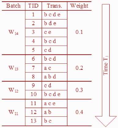
We have the weighted support of the itemset “ cd ” is:

WSWsupp (" cd ") = 0 x 0.4 + 2 x 0.3 + 1 x 0.2 + 3 x 0.1 = 1.1

The minimal weighted support at the time point T 1 :

N

Y = minsupp x f| Wy |xa_y j = 1

• = 20% x (3x 0.4 + 2 x 0.3 + 3 x 0.2 + 5 x 0.1) = 0.58

The WSWsupp (" cd ") = 1.1 >  y = 0.58 , means “ cd” is a weighted frequent itemset over the given data stream. In the other words, we say that the itemset “ cd ” is satisfied by Y .

Definition 4: Mining weighted frequent itemsets over a data stream DS using the sliding window model is finding a set WSW including all weighted frequent itemsets:

WSW = { X/X с I , WSWsupp ( X ) >  y }

Lemma 1 : If X is a weighted frequent itemset then all subset of X are weighted frequent itemsets.

Proof .

We have

DS_X = { T e DS/X с T } is a transaction set including X .

DS_¥ = { T e DS/Y с T } is a transaction set including Y .

Assume that X is a weighted frequent itemset. This means WSWsupp ( X ) >y .

For all subsets Y с X , X ^0 , we have V T e DS_X

> T 2 X 2 Y — T e DSy.

Therefore,

DS_X с DS_¥ ^ \DS_X |< | DS_y|

DS DS

• - F j^{( Y} ) = T DS T > I DS I >  F j^{( X} )

WSWsupp (Y) = ]T F (Y) x a j=1

• > WSWsupp ( X ) = f; F ( X ) x a у

• j =1

Therefore, it is proved that all subsets Y is weighted frequent itemsets.

• IV. Process of Mining Weighted Frequent Itemsets over Data Stream Using Tree Data Structure

Process is given as follows:

• (i)    Building WSWFP-tree (A procedure of building data tree structure);

• (ii)    Mining WSWFP-tree (A Procedure SWFP-miner);

• (iii)    Updating WSWFP-tree by updating window procedure (A Procedure Update Window);

• (iv)    Re-mining WSWFP-tree (Algorithm of mining WSWFP-stream).

• A.    WSWFP-Tree Construction:

As a FP-tree [8,9], a WSWFP-tree has a structural tree and an item table. However, in order to construct a WSWFP-tree, our proposed algorithm has to access entire database one time only. The item table stores all items in the alphabetical order, their weights, the frequence of each item in each batch, and the pointer points to the first node on the WSWFP-tree that has the same name as the first one . The WSWFP-tree involves a root node called a null node (signs as {}) and a set of precedent trees that are subtrees of root node. The transactions of each batch in database are going to insert into WSWFP-tree by their items in alpabetical order. Except root node, each node on WSWFP-tree stores the name of item that the node represents, the frequence of each node in each batch on the branch from root node and pointers point to parents node, children nodes and the node with the same name on the tree.

When a new node is added into a WSWFP-tree by inserting a transaction from batch k of current window including N batches, a list of N frequent values in N batches are filled with the seting of 1 at the position k and 0 at other positions. For instance, if the current window has 4 batches and “ b ” is a node appeares at the first time in the tree by inserting a transaction of batch 2, then the structure of node “ b ” is: 0,1,0,0.

Here is some symbols definition using in each procedure and algorithm.

Table 2. Symbols Definition.

Symbols	Meanings
T,	At point time of z (i=l,2,...)
К	Number of transactions
N	Number of batches
	At point time of T,, and j* batch (i=l,2,...:j=l,2....,N)
№	Size of batch Wtj
	Weight of batch Wy
L	Set of weighted frequent itemset

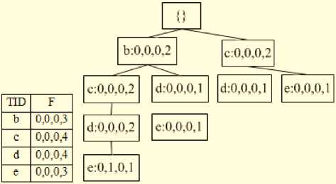
Fig.1. ID Table and WSWFP-tree after Inserting Batch W 14 .

After inserting 4 batches with 13 transactions in Table 1, the resulted ID table and WSWFP-tree can be seen in Fig. 2.

d:0,0,1,0 e:1,0,0,0  d:0,1,1,2  e:0,0,0,1 d:0,1,0,1

Ш)	F
a	2,020
b	2,1,2,3
c	2,2,2,4
d	02,2,4
e	1,1,03

b:1,0,1,0 c:1,0,1,0  c:1,1,1,2  d:0,0,0,1

Input: T , K , N , W_y (i = 1,2,...; j = 1,2,..., N)

Output: WSWFP-tree;

Method

Fig.2. ID Table and WSWFP-tree for all Transaction in Table 1.

• 1.    If (point of T₁) then create a Root, assign a label of Null ({})

• 2.    Scan for (each transaction in current window)

• 3.    Begin

• 4.    With (each transaction т in the j th window) do revise the performing transaction to insert a node to the tree. The method can be seen as follows:

• -    The transactions having the same prefix will go in the same way in the prefix in the WSWFP-tree

• -    Information written in the node will be NameNode ( w₁,w₂,..,w_N ).

• 5.    Build a index table with information as: TID, index, frequent distribution of index in N windows, count of index over stream, pointer pointing to the node that having the same index name in the WSWFP-tree.

• 6.    End;

• 7.    Return WSWFP-tree

If the index in transaction is displayed at the appropriate batch, the w j =1 otherwise, w j =0. If the index is appeared many times, the appropriate w j will be added with 1. Note that, NameNode is a name of tree node, and it also is name of the index over stream.

For example, an index table and WSWFP-tree are created after inserting the batch W 14 (see Fig. 1).

Obviously, the structure of the nodes in the WSWFP-tree store all required information for mining frequent itemsets in a current window of transaction stream. Moreover, a transaction of each batch is traced and updated easily by tracing and updating WSWFP-tree (delete oldfashion transations, add transactions of a new batch) when switching into mining new window.

• B.    Mining A WSWFP-Tree

A WSWFP-tree has important properties, which will be used in the proposal algorithm based on FP-growth approach [8, 9], as follow:

Property 1 : The high of WSWFP-tree equals to the length of the longest transaction.

Property 2 : The sum of frequent values in any node on tree is greater of equal to sum frequent values of any children nodes.

Property 3 : The appeared frequency of an item in each batch equals to summary of corresponding frequent values in all nodes have the same name.

Property 4 : The distribution of frequency in a batch of a branch on the tree is the distribution of frequency of an antecedent node

By applying the FP–growth [8,9], the proposed algorithm called SWFP-miner for mining frequent itemsets with weight over a data stream can be seen as:

Procedure SWFP-miner.

Input :   T , K , N , W ₇, a^( i = 1,2,...; j = 1,2,..., N ), minsupp

• 1.    Calculate the minimal support follows у by (3);

• 2.    From table of items, determine the set C₁ is set of 1 -itemsets satisfy y .

• 3.    L = C ;

• 4.    For each (for each item a in the items’ table, in reverse alphabetical order) do

• 5.    Begin

  • 5.1.    Create the conditional-tree for corresponding item a ;

  • 5.2.    Construct the candidate itemsets;

  • 5.3.    Eiminate the candidate itemsets have the supports do not satisfy y ;

  • 5.4.    Insert the satisfied itemset у into L;

  • 5.5.    Delete all processed node a on conditional-tree;

• 6.    End;
  
  7.    Return L

For example : Given the data in Table 1, at the point time T 1 including 13 transactions and 4 batches as W 11 , W 12 , W 13 , W 14 . The appropriate weights are α 11 =0.4, α 12 =0.3, α 13 =0.2, α 14 =0.1 and the minimal support minsupp is 20%.

Calculate у by (2), there is:

N y = minsupp x ^IW |xa# = 0.58

j = 1

From the item table, count the supports of 1-itemsets are: a : 1.2, b : 1.8, c : 2.2, d :1.4, e :1.0 .

The 1-itemsets satisfy   y =0.58.  Therefore L=C 1

={a,b,c,d,e} .

Construct and extract the condition trees for items in reverse alphabetical order from the bottom of the item table:

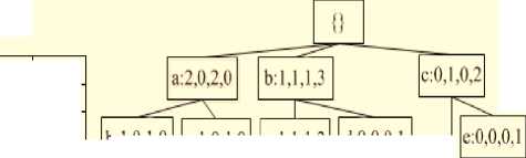
Construct and extract the condition tree of item “e”

Database of condition of the item “ e ” has precedent branch { ac :1,0,0,0; bcd : 0,1,0,1; bd : 0,0,0,1; c : 0,0,0,1 }

From the conditional database, the sub-WSWFP-tree for item “ e ” can be built (see Fig. 3(a)).

From the item table, count the appeared frequencies of two candidates 2-itemsets in the same batch with “ e ” are { ae :1,0,0,0; be : 0,1,0,2; ce : 1,1,0,2, de : 0,1,0,2 } and the supports with weight of the corresponding itemsets are:

ae : 0.4, be : 0.5; ce : 0.9, de : 0.5 . There is an itemsets of " ce " satisfy y . Insert the 2- itemsets of “ ce” into the set L , we have: L = { a , b , c , d , e , ce } .

Continuously extract the 2-itemsets of “ce”. Extract the conditional-tree of itemsets “ce”, Fig. 3(b), there are one candidate 3-itemsets {ace :1,0,0,0} and their weighted supports (ace: 0.4} do not satisfy y. Continue to extract the conditional-tree of the itemsets of “ace” we have a result of null tree. Therefore, L = { a, b, c, d, e, ce}.

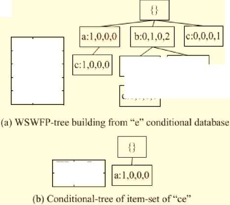
Fig.3. The WSWFP- tree of item “e” and the Conditional-Tree of Itemsets “ce”.

HD	F
a	1,0,0,0
b	0,1,02
c	1,1,02
d	0,1,2,2

HD	F
a	1,0,0,0

с:0,1Д1

d:0,0,0,1

d:0J ,0,1

Construct and extract the condition tree of item “d”

The database of condition of the item “ d ” has some precedent branches as

{ ab : 0,0,1,0; bc :0,1,1,2; b :0,0,0,1; c : 0,1,0,1 }

The database of condition construct WSWFP-tree of the item “ d ” depicted in Fig. 4(a).

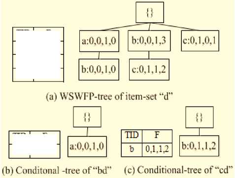
Fig.4. The WSWFP-tree of item “d” and Conditional-Tree of two Itemsets "bd" and "cd".

HD	F
a	o,o, 1,0
b	0,1,23
c	02,13

HD	F
a	0,0,1,0

From the item table with the frequency of item “d”, there are candidates 2-itemsets of "bd" and "cd" satisfy y, according to the windows of {ad :0,0,1,0; bd :0,1,2,3; cd :0,2,1,3} and the appropriate support with weights as ad : 0.2, bd :1.0; cd :1.1 .

Therefore, we have L = { a , b , c , d , e , ce , bd , cd } .

Mining conditional-tree of " bd " (Fig. 4(b)) we have a candidate 3-itemsets of { abd :0,0,1,0 } , and the support with weight of ( abd : 0.2) do not satisfy y .

Mining conditional-tree of " cd " (Fig. 4(c)) we have a candidate 3-itemsets of { bcd : 0,1,1,2 } ? and the support with weight of bbcd :0.7) satisfy y . Inserting " bcd " into L, we have L = { a , b , c , d , e , ce , bd , cd , bcd } .

Continue to mine the conditional-tree of " bcd " we have a null tree.

Therefore, L = [a, b, c, d, e, ce, bd, cd, bed).

Construct and extract the condition tree of item “c”

The database of condition of the item “ c ” has precedent branches { a :1,0,1,0; b :1,1,1, } .

The database of condition construct WSWFP-tree of the item “ c ” depicted in Fig. 5.

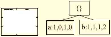
Fig.5. WSWFP-tree Building from Database of "c".

HD	I
a	1,0,1,0
b	1Д,и

At the time point T 1 , the set of weighted frequent itemsets and their supports are

J a :1.2, b : 1.8, c : 2.2, d :1.4, e :1.0, ce : 0.9, bd :1.0, I cd :1.1, bcd : 0.7, ac : 0.6; bc : 1.1; ab : 0.6

• C.    Update WSWFP-Tree by the Use of Update-Window Procedure

To delete the information from oldfashtion batches on a tree, the following tasks have to be done as:

• -    In the list of frequent values of each node on tree, replace the value at first position by 0, and the value at position of j (1< j ≤N) is replace by the value of position of j -1.

• -    Prune any node which has its all frequent values as 0.

After deleting the oldfashion batches, a new batch is inserted in to the tree as normal (call Procedure ConstructWSWFP-tree) .

For example : Fig. 7 represents a WSWFP-tree at the point time T 1 after deleting the batch W 14 .

Asume that at the point time T 2 , the window of data stream can be seen in Table 3.

After deleting the old fashion batches, the transactions of new batch are inserted into tree and a new update tree at the point time T 2 can be seen in Fig. 8.

Do the same method as constructing and extract of other items above we have:

L = { a , b , c , d , e , ce , bd , cd , bcd , ac ; bc } .

Construct and extract the condition tree of item “b”

The database of condition of the item “ b ” has one precedent branch { a :1,0,1,0 } .

The database of condition construct WSWFP-tree of the item “ b ” depicted in Fig. 6.

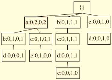
Fig.7. WSWFP-tree after Deleting Batch W14 with Database in Table 1.

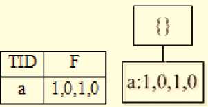
Fig.6. The WSWFP-tree of item “b”.

Do the same method as constructing and extract of other items above we have:

L = { a , b , c , d , e , ce , bd , cd , bcd , ac ; bc ; ab } .

Construct and extract the condition tree of item “a”

The result is a null tree.

Table 3. An Example of Data Stream at Time-Point T2.

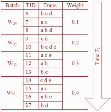
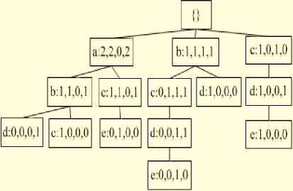
Fig.8. WSWFP-tree after Updating Batch of W21 at Time-Point T2.

• 1.    For each (route in WSWFP-tree) do

• 2.     Begin

• 3.    With (current node) then change Its values as: NameNode ( w , w₂ ,..., w ^)   is replaced by

• 4.    If (for all ■w = 0 ) then delete the nodes in the

• 5.     End ;

• 6.    Scan for (all transactions in the new batch ( W ))

• 7.    Begin

• 8.    Call ConstructWSWFP-tree ; // Only perform over transactions in the newest batch;

• 9.    End;

• 10.    Return WSWFP-tree

NameNode (0, w ,..., w ^ );

route;

D. Mining Frequent Data-Set with Weights over Data Stream by Using Tree

The algorithm WSWFP-stream is built basing on mining many time the data stream in WSWFP-tree (delete the old fashion window and update the new one in the 3rd step).

Input : T , K , N , W_o , a^ ( i = 1,2,...; j = 1,2,..., N ), minsupp;

• 1.    If (point of T ) then

• 2.    Begin

• 3.    Call ConstructWSWFP-tree ;  // Building a tree with

• 4.    Call SWFP-miner ; // Mining WSWFP-tree for the first time

• 5.    End
  
  6.    Else
  7.    Begin

• 8.     cont=”Y”;

• 9.    While (upper(cont)=”Y”) do // Process will be

• 10.   Begin

• 11.    Call ReleaseWindowOld ; //Delete the oldfashion windows

• 12.    Call UpdateWindow ;

• 13.    Call SWFP-miner ;    // Re-mining WSWFP-tree

• 14.    Accept “Do you want to mine data stream (Y/N)?” to cont;

• 15.    If (upper(cont)≠”Y”) then exit;

• 16.   End ;

• 17.    End;
  
  18.    Return L

• 19.   End .

all transactions over data stream

repeated with variable of cont

(after updating)

• V.    Experiment

  In order to evaluate the performance of WSWFP-stream and compare to the Tsai's two algorithms (WSW and WSW-Imp), we have run several tests on PC Pentium dual core 2.13 GHz CPU with 1GB memory of the use operating system Window 7. The program is coded by Microsoft Visual C++ version 6.0, and method to generate transactions has been done the same as one used in Apriori [2]. The given parameters for the experiment as: the number of items N = 1000, and the maximum number of frequent itemsets |L| = 2000.

To simulate a data stream as a weighted sliding window model, each transaction is processed continuously. We also assume that the number of transactions in each batch is the same. In our experiment, the number of transactions in each batch is 4, and the weights of each batch W_{i 1}, W_{i 2}, W_{i 3} and W_{i 4} are 0.4, 0.3, 0.2 and 0.1, while the weight w_{i 1} is closest window of present time point i .

Fig. 9 shows the processing times of three algorithms WSWFP-stream, WSW and WSW-Imp with different minimal supports. In this test, the total number of transactions is 100K and the number of each batch is 10K. Because the number of batches in each window is 4 then the number of time points is 7. The processing time is summary of times spent for all time points.

In overall, it shows that the WSWFP-stream running time is better in alternative minimal supports. For example, WSWFP-stream running time is taken in about 27 seconds whereas WSW and WSW-Imp running time are over 32 seconds.

The figure shows that as the minimal support reduces the competitive advantage of WSW-Imp increases.

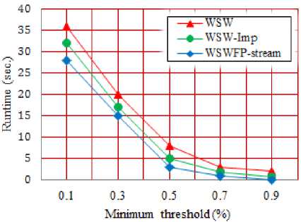
Fig.9. The Processing Times of Three Algorithms Vs the Minimal Support.

Fig. 10 depicts the processing times of three algorithms WSWFP-stream, WSW and WSW-Imp with different number of transactions in a sliding window at minimal support value 0.1. The processing times of three algorithms are increase as the number of transactions increase. The WSWFP-stream running time is nearly the same as two others at the small number of transaction. However, its running is quite different to the others when the number of transactions are increased. For example, with 250K of transaction the WSWFP-stream running time was taken in 90 seconds whereas the others running times were more than 100 seconds. In overall, the performance of WSWFP-stream is out standing from the two algorithms, WSW and WSW-Imp, in all situations.

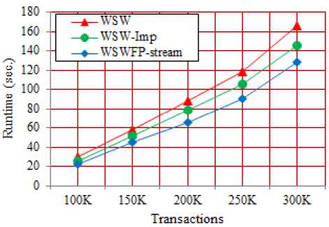
Fig.10. The Processing Time Vs the Number of Transactions in a Sliding Window.

To compare the results of three algorithms, we have been experimented them to alternative size of batch.

The Fig. 11 shows the effect of size of batch, from 1K to 20K of transactions, at the minimal support 0.5. We can see that as the size of a batch increases the different between the processing times of three algorithms WSWFP-stream, WSW and WSW-Imp decreases.

For example, for 1K size of batch, the WSWFP-stream running time is taking in advance but its time is going to the same as WSW and WSW-Imp running times at the large size (over 20K).

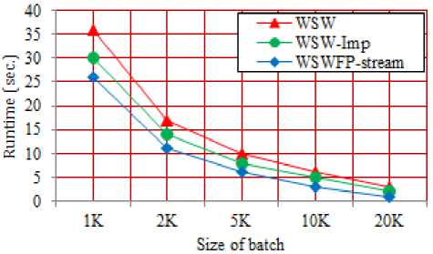
Fig.11. The Processing Time Vs The Size of Batch.

When the size of batch is small the number of frequent itemsets is small also that cause the probability of infrequent itemsets in a batch is higher. In general, the performance of WSWFP-stream algorithm is better than the performances of two algorithms WSW and WSW-Imp.

• VI. Conclusion

The mining frequent itemsets has an important role in data mining to mine the data n the real world. In this paper, basing on the weighted sliding window model derived from Tsai P. S. M. [20], we have proposed a new algorithm so-called WSWFP-stream for mining weighted frequent itemsets over a data stream. This algorithm is based on the FP-growth’s approach [8,9]. It means that the algorithm's process only needs to access the database one time, stores all information in a tree, which has an easily updating structure and does not generate large number of candidates during the extraction. Therefore, the proposed algorithm WSWFP-stream is theoretically more efficient than Tsai's algorithms (WSW and WSW-Imp) in processing time and memory aspects. The experiment also proved this point of view.