An Efficient Dimension Reduction Quantization Scheme for Speech Vocal Parameters

Author: Qiang Xiao, Liang Chen, Ya Wang
Journal: International Journal of Information Technology and Computer Science(IJITCS) @ijitcs
Article in issue: 1 Vol. 3, 2011.
Free access
To achieve good reconstruction speech quality in a very low bit rate speech codecs, an efficient dimension reduction quantization scheme for the linear spectrum pair (LSP) parameters is proposed based on compressed sensing (CS). In the encoder, the LSP parameters extracted from consecutive speech frames are shaped into a high dimensional vector, and then the dimension of the vector is reduced by CS to produce a low dimensional measurement vector, the measurements are quantized using the split vector quantizer. In the decoder, according to the quantized measurements, the original LSP vector is reconstructed by the orthogonal matching pursuit method. Experimental results show that the scheme is more efficient than that of conventional matrix quantization scheme, the average spectral distortion reduction of up to 0.23dB is achieved in the DFT transform domain. Moreover, in the approximate KLT transform domain, this scheme can obtain transparent quality at 5 bits/frame with drastic bits reduction compared to other methods.
Low bit rate speech coding, Line Spectrum Pair (LSP), Compressed Sensing (CS), Discrete Fourier Transform (DFT), Karhunen-Loeve Transform (KLT)
Short address: https://sciup.org/15011603
IDR: 15011603
Text of the scientific article An Efficient Dimension Reduction Quantization Scheme for Speech Vocal Parameters
Published Online February 2011 in MECS
Many low bit rate speech coding algorithms are based on Linear Predictive Coding (LPC) and the LSP parameters are chosen for representing LPC coefficients. For the LP based vocoders such as MELP or MELPe, the bits used for quantizing LSP parameters have already taken up to 60% [1], so the bit rate reduction is strongly tied to efficient quantization of LSP parameters.
The transparent Scalar Quantization (SQ) of LSP parameters requires typically 38 to 40 bits/frame [2]. Lower bit rates can be achieved using the Vector Quantization (VQ). VQ considers the entire set of LSP parameters as an entity and allows for direct minimization of quantization distortion. Accordingly, VQ results in smaller quantization distortion than the SQ at any given bit rate, it provides 1 dB average spectral distortion using about 26 to 30 bits/frame [3,4]. However, for transparent quantization performance, VQ needs a large number of codevectors in its codebook, it means that the storage and computational requirements for VQ are prohibitively high. It’s known that there is high correlation between two neighbouring LSP frames, and between adjacent LSP parameters within a frame, so the bit rates can be further reduced when both interframe and intraframe redundancy is removed. The exploitation of intraframe redundancy usually use the Split Vector Quantization (SVQ) [5] and Multi-Stage Vector Quantization (MSVQ) [6], which offer transparent quantization performance with realistic codebook storage and search characteristics at 22 to 24 bits/frame. Further compression can be obtained in principle by exploiting interframe correlation between sets of LSP parameters. In this way, the Predictive Vector Quantization (PVQ) [7,8] and Matrix Quantization (MQ) [9,10] systems have been proposed, which offer high quantization accuracy at 18 to 21 bits/frame.
Now, there are more advanced efforts to lower the speech coding bit rates below 600bps. However, with the bit rates reduce, the number of consecutive frames which are grouped together becomes larger. Such a multi-frame structure has the two following problems. Firstly, a large codebook requires prohibitively large amount of training data and the training process can take much of computation time. Secondly, the encoding complexity and storage requirement increase dramatically, and the quantization performance degrades as the bits per frame are further reduced.
To overcome these drawbacks, a novel LSP parameters quantization scheme based on compressed sensing (CS) is proposed in this paper. The recent studies of CS have shown that sparse signals or compressible on some basis can be recovered accurately using less observations than what is considered necessary by the Nyquist/ Shannon sampling principle [11,12,13,14]. Based on this theory, CS sampling and reconstruction of LSP parameters on the DFT and KLT transform domain are realized. In the encoder, the LSP parameters extracted from consecutive speech frames are grouped into a high dimensional vector, and then the dimension of the vector is reduced by CS to produce a low dimensional measurement vector, the measurements are quantized using the split vector quantizer. In the decoder, from the quantized measurements, the original LSP vector is reconstructed by the Orthogonal Matching Pursuit (OMP) method [15]. Experimental results indicate that this novel quantization scheme can obtain higher performance than MQ while in the DFT domain. Furthermore, in the KLT domain, the scheme can obtain transparent quality at 5 bits/frame with realistic codebook storage and search complexity.
The rest of this paper is organized as follows. In section II, basic principles of compressed sensing are introduced. In section III, the compressed sensing formulation for LSP parameters is proposed. In section IV, the quantization scheme is designed. Then simulation results are presented and discussed in section V. Finally, we give out the conclusion.
-
II. C OMPRESSED S ENSING PRINCIPLES
Compressed sensing is a newly introduced concept of signal processing which aims at reconstructing a sparse or compressible signal accurately and efficiently from a set of few non-adaptive linear measurements.
Let X e R N x 1 be a real-valued signal of length N , assume that X is k -sparse or compressible on a particular orthonormal basis Y = { ф , ф 2,••• ф N } , Y e RN x N i.e. X can be represented as:
N
X = Y® = £ фi9i (1) i=1
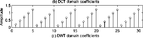
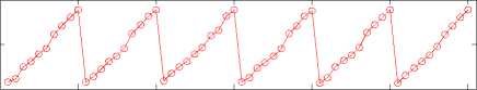
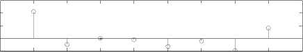
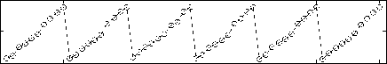
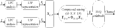
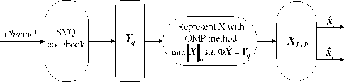
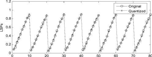
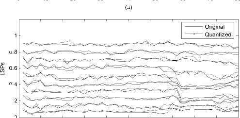
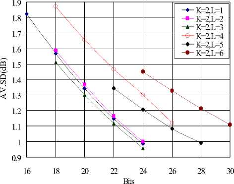
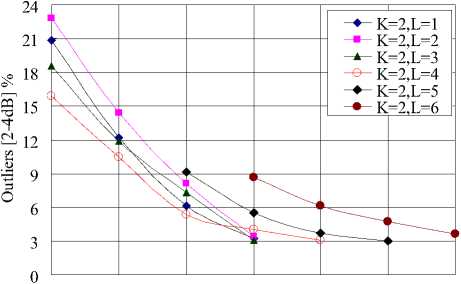
Where 0 = {^, ft ,...^ }T is a scalar coefficient vector 1 2 N of X in the orthobasis. X and ® are equivalent representations of the signal, with X in the time domain and ® in the Y domain. The assumption of sparsity means that only k nonzero coefficients, with k Y = фX = фY® (2) Where Ф e RMxN is a measurement matrix made up of random orthobasis vectors, Y e RMx1 is called the measurement vector of original signal. CS theory states that we can reconstruct X accurately from Y if Ф and Y are incoherent, this property is easily achieved when the entries of random matrix Ф are i.i.d. Gaussian variables. If the incoherence holds, the following linear program gives an accurate reconstruction with very high probability: ® = argmin 1|®|| 0 s.t. Y = ФY0 (3) Where 0 is the l0 norm. Unfortunately, the above optimization problem is NP-hard and can not be solved efficiently. Recently, it has been shown that if the sensing matrix Ф obeys a so-called restricted isometry property (RIP) [14] while ® is sparse enough, the solution of the combinatorial problem (3) can almost always be obtained by solving the constrained convex optimization: ® = argmin ||®|| 1 s.t. Y = ФY® (4) The convex l1 norm minimization problem can be solved with the traditional linear programming techniques. However, these techniques are still somewhat slow. At the expense of slightly more measurements, fast iterative greedy algorithms have been developed to recover the signal. Examples include the Orthogonal Matching Pursuit (OMP) [15] and tree matching pursuit methods. Once the optimal solution ® is got, the signal X can be recovered by: N X Y® = ^фД (5) i=1 Summarizing, if we wish to use CS to compress LSP parameters, three main ingredients are needed: a domain where the LSP parameters is sparse, the measurement matrix and the reconstruction algorithm. In the next section, we will give a detailed analysis of the compressed sensing formulation for LSP parameters. III. COMPRESSED SENSING FORMULATION FOR LSP A. LSP parameters representation Consider the LPC analysis is applied to speech frames of D ms duration to yield the coefficient vectors a(") = [a",a",...,a”], where p is the order of the LPC filter and n is current LPC analysis frame, a(n) is then transformed to a LSP representation l(") =[l”,l",...,l”]. When performed over L consecutive speech frames provides an L-by-p matrix: X= Г l1 1 n +1 M г l2 n+1 M f lP n+1 lP M , n +L-1 n+L-1 n+L-1 lp L×p Let N=L×p, the above matrix is then shaped into an N dimensional column vector: X = [ 11" -lp" 11"+L-1... lp+ L-1]T [l 1,12 , •••*,1 n ] B. Sparse representation of LSP In this section, we will discuss some important issues in applying CS to LSP parameters. First, we need to know which domain of LSP is sparse, it is the precondition of applying CS to LSP parameters. Several experiments are conducted to examine the Discrete Fourier Transform (DFT) domain, the Discrete Cosine Transform (DCT) domain, the Discrete Wavelet Transform (DWT) domain and the Karhunen-Loeve Transform (KLT) domain, we find that the LSP parameters are sparse in the DFT and KLT domain. Here, we give the definition of the DFT and KLT transform domain. As the DFT transform domain is well known in digital signal processing, so there is no need to give a detailed analysis. The KLT is an efficient data compression technique, which has been successfully used to extract the data features. The bases of the KLT are the eigenvectors of the autocorrelation matrix. Assuming that Rx is the autocorrelation matrix of the signal X, when the KLT is calculated over the vector X, the Rx can be estimated by: Rx -{ XX") Let U be a matrix whose columns constitute a set of orthonormal eigenvectors of Rx , so that UUT = I and: Rx = UЛUT Where Λ is the diagonal matrix of non-null eigenvalues: Л = diag (X p X 2,..., X k) (10) For every vector X, through the matrix UT , we can obtain the sparse coefficients vector 0 as: 0 = UT X (11) Unfortunately, the KLT requires much of computation time for the eigenvector decomposition, some approximated approaches to overcome this problem have been developed [16,17]. Furthermore, in practice, we can limit the length of LSP parameters in a reasonable range. As a practical example in Fig.1, when the 60 dimensional LSP parameters extracted from six successive speech frames are transformed into the DFT, DCT, DWT and KLT domain, we find that the coefficients of the DFT and KLT domain are sparse, it is clearly shown that the LSP signal is compressible in the DFT and KLT domain. < 0 10 20 30 40 50 60 (a) DFT domain coefficients 4 10 20 30 40 50 60 E 0 10 20 30 40 50 60 (d) KLT domain coefficients Figure 1. The transform domain of LSP parameters Once we find the sparse domain, another issue with LSP parameters is the sparsity. We know that the sparsity k means that the number of nonzero coefficients in Θ which are sufficient to represent X. As in Fig.1, it is clearly shown that there are only 10 obvious nonzero coefficients in the DFT domain, while in the KLT domain, there is only 1 obvious nonzero coefficient, all the other coefficients are zero or closes to zero. Moreover, in the KLT domain, we can use a heuristic choice of K=k+1 when the improvement in the accuracy of the reconstruction is achieved. So we can reasonably assume that the sparsity k in the DFT domain is 10, in the approximated KLT domain is 2. C. Sensing LSP with the Gaussian random matrix The measurement matrix must allow the reconstruction of the length-N signal X from M<N measurements. Since M< N, this problem appears ill-conditioned. However, X is k-sparse and the k locations of the nonzero coefficients in Θ are known, then the problem can be solved efficiently. When using CS, one must choose how many samples to retain. As a rule of thumb, four times as many samples as the number of non-zero coefficients should be used [18], i.e., M=4k. Now, it is clear that the size of the measurement matrix Φ depends uniquely on the sparsity level k. Meanwhile, for the effective CS reconstruction, Φ and Ψ must be incoherent, this property can be achieved when the measurement matrix Φ constructed from independent and identically distributed zero-mean Gaussian variables. Consequently, the Gaussian random matrix is used as the measurement matrix throughout the paper. D. LSP recovery with OMP Although the quality of the reconstruction mainly depends on the compressibility of LSP parameters, the reconstruction algorithm is also very important. As mentioned in section II, the Orthogonal Matching Pursuit (OMP) algorithm is an attractive method for the sparse signal recovery. OMP is a fast greedy algorithm that iteratively builds up a signal representation by selecting the atom that maximally improves the representation at each iteration. The OMP is easily implemented and converges quickly, which is chosen for the LSP recovery. E. Realization of CS processing In Fig.2, a practical example of CS recovery of LSP parameters is illustrated. Consider 60 dimensional LSP parameters (Fig.2(a)) extracted from 6 constructive speech frames, when transformed into the approximate KLT domain, the sparsity k is 2, then with the relation M=4k, 8 measurements (Fig.2(c)) are obtained. According to the 8 measurements, the original LSP parameters can be reconstructed by the OMP method. We clearly see that the reconstruction works very well, the recovered LSP signal (Fig.2 (d)) match the original signal with very high accuracy. 0 10 20 30 40 50 60 (a) the original LSP Е 0 10 20 30 40 50 60 (b) the sparse coefficients Е -5 (c) the measurements 0.5 Е 0 10 20 30 40 50 60 (d) the reconstructed LSP Figure 2. Example of CS recovery of LSP parameters in the KLT domain (L=6, k=2) Since the LSP parameters can be compressed and recovered efficiently by the compressed sensing, if, however, we encode the low dimensional measurements instead of the original LSP signal, the coding bit rates can be definitely reduced. In other words, the quantization performance will much improved under the same coding bits as used in other methods. IV QUANTIZATION SCHEME Based on the above analysis, a Compressed Sensing Vector Quantization (CSVQ) scheme for LSP parameters is proposed in this section. Fig.3 shows a block diagram of the CSVQ quantization system. Here, the pth (p=10) order linear prediction analysis is performed on D ms speech frame, the LSP parameters extracted from L successive frames are gathered up to form a matrix, the matrix is then converted into a N dimensional column vector. (a) Encoder (b) Decoder Figure 3. CSVQ encoding and decoding process The quantization procedure is summarized as follows: 1) Compressed sensing: the original LSP parameters are sensed by the measurement matrix Φ according to (2), once X has been measured, the high dimensional LSP parameters X can be converted into a low dimensional measurement vector Y. 2) Quantizing the measurement vector Y with SVQ: in CSVQ, to reduce the coding bit rates, the low dimensional measurement vector Y is quantized instead of the original LSP signal. Here, the Split Vector Quantizer is utilized to quantize the measurements. As mentioned above, in the DFT and KLT domain, the sparsity k is 10 and 2, respectively. After compressed sensing, according to the empirical rule of thumb, four times as many samples as the sparsity is achieved, i.e. there are 40 and 8 measurements need to be quantized, respectively. To moderate the complexity and performance, in SVQ, the 40 measurements in DFT domain is split up into 4 subvectors, each subvector has 10 measurements and equally quantized with 10 bits. In the KLT domain, the 8 measurements are split up into 2 subvectors, the first subvector has the first 4 measurements and the second subvetor has the remain 4 measurements. For minimizing the complexity of the SVQ, total bits available for measurements quantization are divided equally to each of the two subvectors. The total squared error (or Euclidean) distance measure is used for the SVQ operation both in the DFT domain and KLT domain. The codebooks are designed using the well-known LBG algorithm to minimize the error distance based on a sufficiently rich training sequence. 3) Send: the index of quantized measurements Yq is communicated to the receiver. 4) LSP recovery with OMP: in the decoder, we consider the problem of recovering sparse signal X from a set of quantized measurements Yq . The quantized measurements are found according to the corresponding index of the codebook. Once Y has been quantized, the reconstruction of LSP parameters involves trying to recover the original LSP signal by the OMP method. The recovered LSP signal is the ultimate quantization value of the original LSP signal. V EXPERIMENT RESULTS Several experiments are conducted to examine the performance of the proposed CSVQ method, we start with the discussions on the simulation setup. All experiments are based on the TIMIT speech database, down sampled to 8 kHz. A 10th order LPC analysis using the autocorrelation method is performed on every 20 ms speech frame. A fixed 15 Hz bandwidth expansion is applied to each pole of the LPC coefficient vector, and finally the LPC vectors are transformed to the LSP representation. The corresponding CSVQ codebooks are designed using the training data consist of 2×10⁷ speech frames, in addition, about 2×10⁵ speech frames that out of the training speech are used to evaluate the performance. Traditionally, the objective measure that is used to assess the performance of quantization scheme is the Spectral Distortion (SD) measure: N 1 1π SD= ∑ [10log10Sn(ω) -10log10Sn(ω)]2dω (12) N n=1 π 0 10 n 10 n Where N is the frame number used for SD calculation, the Sn (ω) and Sˆn (ω) are the original and quantized LPC power spectrum, respectively. A. CSVQ performance in the DFT transform domain To evaluate the performance of CSVQ in DFT domain, three methods are compared: the split matrix quantization (SMQ), the multi-stage matrix quantization (MSMQ) and the CSVQ. In SMQ, 8 consecutive speech frames provide a LSP matrix (SMQ-8), the matrix is split up into 4 submatrices, and each submatrix is quantized with 8 bits. In MSMQ, the LSPs from 8 successive frames are gathered up to form a matrix (MSMQ-8), which is quantized with four stage codebook of 256, 256, 256, 256 levels, respectively. In CSVQ, the LSPs from 8 and 10 consecutive frames are grouped into a high dimensional vector, denoted as CSVQ-8 and CSVQ-10, respectively. The 40 dimensional measurements is split up into 4 subvectors, each subvector is quantized with 10 bits. The quantization results are given in table I. TABLE I. COMPARISON OF THE SD PERFORMANCE Quantization scheme Bits/frame AV. SD (in dB) Outliers (in %) 2-4 dB > 4 dB SMQ-8 4 3.4661 66.26 25.61 MSMQ-8 4 3.3408 67.15 24.46 CSVQ-8 5 3.1757 56.34 22.87 CSVQ-10 4 3.2752 58.29 24.36 As can be seen, in the DFT domain, the CSVQ-8 provides an average SD value of 3.1757 dB, which is smaller than SMQ-8 and MSMQ-8, the average reduction of AV.SD is up to 0.23 dB, and the percentage of outlier is smallest among all the quantization schemes. CSVQ-10 gives an average SD value of 3.2752 dB, which is slightly higher than CSVQ-8, the reason is that the reconstruction error becomes higher with the dimension of LSP parameters increases while at the same sparsity. Fig.4 illustrates the original LSP parameters and the quantized results obtained by CSVQ, we can see that quantized value matched with the original signal quite well. (a) 0.4 0.2 (b) 0 0 40 60 frames Figure 4. Comparison of original and quantized LSPs in DFT domain (L=8, k=10) (a) A superframe LSPs; (b) Trajectories of LSPs Although the CSVQ performance of the DFT domain is better than the matrix quantization scheme, it is necessary to point out that the average SD value is still over 3.0 dB when the quantization rate below 250bps. However, if we find a sparser domain than the DFT, the CSVQ performance can be further improved. In the next section, we will see the transparent quantization performance can be achieved while in the KLT domain. B. CSVQ performance in the KLT transform domain In the KLT domain, the proposed CSVQ approach is simulated for different values of L (1-6) and quantization bits (16-30). No matter how many successive frames are gathered up, there are only 8 measurements need to be quantized. In CSVQ, the 8 measurements are always quantized using the SVQ method, which are split up into 2 subvectors, and each subvector is quantized with 8 to 15 bits. The spectral distortion and outlier results for the CSVQ are shown in Figs. 5 and 6. For the transparent quantization performance, a single frame of CSVQ needs 24 bits, which is comparable with the SVQ [5]. However, an increase of L from 2 to 3, the CSVQ totally needs 24 bits, i.e. with L=2 and L=3, the CSVQ operates transparently at 12 bits/frame and 8 bits/frame respectively. Whereas a further increase to L=4 totally needs 26 bits (6 bits/frame), L=5 totally needs 28 bits (5.6 bits/frame) and L=6 totally needs 30 bits (5 bits/frame). As can be expected, the total quantization bits used for transparent performance are increased with the L increase, the reason for this correlation is that the reconstruction error of CS becomes higher with the dimension of LSP parameters increase while at the same sparsity. To show the benefit of CSVQ in the KLT domain, comparing the results of CSVQ with other methods. For transparent quantization performance, the traditional SVQ needs 24 bits/frame [5], the MSVQ needs 22 bits/frame [6], the MSMQ needs 18 bits/frame [9]. However, in CSVQ, it is only used 5 bits/frame, the drastic bits reduction is achieved compared to other methods. Figure 5. The Average Spectral Distortion of CSVQ in KLT domain TABLE П. THE SD PERFORMANCE IN KLT DOMAIN Quantization scheme Bits/frame AV.SD (dB) Outliers (%) 2-4 dB > 4 dB SVQ 24 1.0320 3.30 0.03 MSVQ 22 1.0400 3.54 0.04 MSMQ 18 1.1000 3.42 0.05 CSVQ (L=1) 24 0.9860 3.19 0.03 CSVQ (L=2) 12 0.9913 3.38 0.07 CSVQ (L=3) 8 0.9584 3.06 0.36 CSVQ (L=4) 6 1.1005 3.10 0.34 CSVQ (L=5) 5.6 0.9905 3.31 0.12 CSVQ (L=6) 5 1.1090 3.64 0.21 20 22 24 26 28 30 Bits Figure 6. Outlier performance of CSVQ in KLT domain Table II shows the detail SD performance. According to the test results, when we consider the average and outlying SD performance, we can see that the performance of the combination from 24 bits/frame to 5 bits/frame is comparable to each other. As the number of successive frames L increase, the bits used for per frame decrease. There are good intuitive reasons to believe that increasing the value of L will lead to improved investigation of the potential of the compressed sensing. However, if a further increase to L=7, the CSVQ can obtain a SD very near 1 dB at a rate of 34/7 bits/frame with a low percentage of outliers. However, at 34 bits, the codebook storage and search complexity are too high to acceptable. In particular, we notice that there are two main factors involved in CSVQ that influence the spectral distortion, one is the reconstruction error of the CS, and the other is the quantization distortion of the measurements. However, the reconstruction error in the KLT domain is far less than the quantization distortion. Increasing the number of measurements can definitely reduce the reconstruction error, however, with a cost of increased storage requirements and search complexity. Taking L=7 as a practical example, when k=2, after CS, there are 8 measurements, with 28 bits for quantization, the AV.SD is 2.0306 dB. While k=3, there are 12 measurements, with 28 bits for quantization, the AV.SD is 1.6199 dB. The two combinations are uniformly quantized with the same bits, the higher k leads to a smaller SD however at expense of increasing complexity. C. Codebook storage and search complexity Table III illustrates the codebook storage and search complexity in different CSVQ configurations. Assume that the CSVQ has m subvectors, each subvector with n measurements is quantized using j bits, thus the total number of codebook elements is equal to m×2j×n. The search complexity is defined as the number of arithmetic operations to obtain the quantized measurements [6], which is typically presented on the logarithmic scale. As shown in table III, the simulation results clearly show that the CSVQ complexity characteristics are directly proportional to the storage requirements. The better performance is achieved however at the expense of slightly increasing the storage requirements and search complexity. Meanwhile, the increase in storage and complexity should pose no problems with the modern DSP processor. TABLE Ш. CODEBOOK STORAGE AND SEARCH COMPLEXITY Quantizer Codebook storage (KWords) Search complexity (MIPS) Traditional quantization methods SVQ 40.9600 16.9069 MSVQ 51.2000 17.1087 SMQ-8 20.4800 15.9100 MSMQ-8 81.9200 18.7200 CSVQ in the DFT transform domain CSVQ-8 40.9600 17.0500 CSVQ-10 40.9600 17.0800 CSVQ in the KLT transform domain CSVQ (L=1) 32.7680 16.5850 CSVQ (L=2) 32.7680 16.5850 CSVQ (L=3) 32.7680 16.5850 CSVQ (L=4) 65.5360 17.5850 CSVQ (L=5) 131.072 18.5850 CSVQ (L=6) 262.144 19.5850 VI CONCLUSION In this paper, we have presented a novel and efficient quantization scheme for quantizing the LSP parameters at low bit rates. This is the first time the ideas of compressed sensing are applied to represent the LSP parameters. The proposed technique involves dimensional reduction and quantizer design two parts. Simulation results show that the proposed CSVQ can give better performance compared with conventional Matrix Quantization schemes in the DFT domain. Furthermore, in the KLT domain, the scheme can obtain transparent quantization performance at 5 bits/frame with realistic codebook storage and search complexity. Meanwhile, the performance can be further improved by finding more accurate ways to reconstruct the LSP parameters or quantizing the measurements more efficiently. ACKNOWLEDGMENT The authors wish to acknowledge the financial support of National Natural Science Foundation of China under grant 61072042.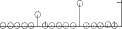
References An Efficient Dimension Reduction Quantization Scheme for Speech Vocal Parameters
- G.Gwénaël, C.François, R.Bertrand, et al. New NATO STANAG narrow band voice coder at 600bits/s. IEEE ICASSP 2006, pp.689-692.
- I.A.Gerson, M.A.Jasiuk. Vector sum excitation linear prediction (VSELP) speech coding at 8 kbps. IEEE ICASSP 1990, pp.461-464.
- T.Moriya, M.Honda. Speech coder using phase equalization and vector quantization. IEEE ICASSP 1986, pp.1701-1704.
- Y.Shoham. Cascaded likelihood vector coding of the LPC information. IEEE ICASSP 1989, pp.160-163.
- K.K.Paliwal, B.S.Atal. Efficient vector quantization of LPC parameters at 24bits/frame. IEEE Trans. on speech and audio processing, Vol. 1, No. 1, pp.3-14, 1993.
- W.P.LeBlanc, B.Bhattacharya, S.A.Mahmoud, et al. Efficient search and design procedures for robust Multistage VQ of LPC parameters for 4 kb/s speech coding. IEEE Trans. on speech and audio processing, Vol. 1, No. 4, pp.373-385, 1993.
- Xia Zou, Xiongwei Zhang. Efficient coding of LSF parameters using multi-mode predictive multistage matrix quantization. IEEE ICSP 2008, pp.542-545.
- S.Subasingha, M.N.Murthi, S.V.Andersen. On GMM kalman predictive coding of LSFs for packet loss. IEEE ICASSP 2009, pp.4105-4108.
- S.özaydin, B.Baykal. Matrix quantization and mixed excitation based linear predictive speech coding at very low bit rates. Speech communication, Vol. 41, pp.381-392, 2003.
- Xia Zou, Xiongwei Zhang, Yafei Zhang. A 300bps speech coding algorithm based on multi-mode matrix quantization. IEEE WCSP 2009, pp.1-4.
- D.L.Donoho. Compressed sensing. IEEE Trans. on information theory, Vol. 52, No. 4, pp.1289-1306, 2006.
- T.V.Sreenivas, W.B.Kleijn. Compressed sensing for sparsely excited speech signals. IEEE ICASSP 2009, pp.4125-4128.
- R.G.Baraniuk. Compressive sensing. IEEE Signal Processing Magazine, Vol. 24, No. 4, pp.118-121, 2007.
- E.Candès, T.Tao. Decoding by linear programming. IEEE Trans. on information theory, Vol. 51, No. 12, pp.4203-4215, 2005.
- J.A.Tropp, A.C.Gilbert. Signal recovery from random measurements via orthogonal matching pursuit. IEEE Trans. on information theory, Vol. 53, No. 12, pp.4655-4666, 2007.
- C.E.Davila. Blind adaptive estimation of KLT basis vectors. IEEE Trans. on signal processing, Vol. 49, No. 7, pp.1364-1369, 2001.
- F.Gianfelici, G.Biagetti, P.Crippa, et al. A novel KLT algorithm optimized for small signal sets. IEEE ICASSP 2005, pp.405-408.
- A.Zymnis, S.Boyd, E.Candès. Compressed sensing with quantized measurements. IEEE Signal Processing letters, Vol. 17, No. 2, pp.149-152, 2010.
