An Efficient Machine Learning Based Classification Scheme for Detecting Distributed Command & Control Traffic of P2P Botnets

Published Online November 2013 in MECS DOI: 10.5815/ijmecs.2013.10.02

• II.    Related works

• III.    PROBLEM DESCRIPTION AND ASSUMPTIONS

The modern network traffic involves various data types, such as files, e-mails, Web contents, real-time audio/video data streams, etc. Each of these data types either use TCP or UDP as transport layer protocol depending on the type of transmission needed. For example, for transfer of files, e-mails, Web contents etc., the Transmission Control Protocol (TCP) appears to be suitable for its reliability. On the other hand, for transfer of real-time audio/video data streams, which is timesensitive, the User Datagram Protocol (UDP) is typically used. Applications using TCP establishes full-duplex communication and also flow control i.e. while establishing connection, the ACK sent back to the sender by the receiving TCP, indicates to the sender the number of bytes it can receive beyond the last received TCP segment, without causing overrun and overflow in its internal buffers. Most P2P applications use UDP protocol for communication. Therefore, when we capture data from various applications in the internet, we find non uniformity in terms of volume, time etc. and in many cases are also unidirectional in nature.

• IV.    ARCHITECTURAL OVERVIEW AND DATA SET PREPARATION

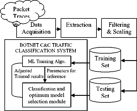
Description of the pipeline diagram:

• i)    Data Acquisition: Raw packets were collected using Wireshark[22] from different computers connected to our campus network. We acquired the botnet dataset of Nugache bot from Department of Computer Science, The University of Texas at Dallas. This is the same dataset which were used in the botnet related research works of [23].

• ii)    Extraction: Useful features for classification were extracted from packet headers. We extracted different kind of information from packet data like the size of largest packet transferred in a flow, the ratio of this packet in a given flow, the difference in time (calculated in seconds) for last packet received in either direction for responding flows, difference in number of packet being sent in either direction for responding flows and also several other features extracted from packet headers. For non-responding flows we include a unique number(we consider a very large number) to make it differentiable. We used 999 for difference in number of packets and 99999 for difference of time. However, more than 60% of normal traffic flows in our dataset has responding flows.

• iii)    Filtering & Scaling: We filtered our datasets through removal of unwanted flows so that it is optimized for classification. We removed the flows having a single packets , since single packets does not provide any statistically significant information. Similarly, flows representing NetBIOS services, broadcasting and DHCP were removed. We scaled the datasets to the range of 0 to 1. We created three separate files containing 18926, 18898 and 18826 instances. Each file contains flow captured for more than 10 hours for each bot as well as normal web traffic. Normal network flows comprised 17.83 % of total flows on an average of the three files.

• iv)    Botnet C&C traffic classification system: We feed our optimized datasets to our Botnet C&C traffic classification using 10 fold croos validation. The botnet C&C traffic classification system has two modules – one for training the system using input training sets and the other to evaluate the optimum model using testing set.

• V.    CLASSIFICATION AND ANALYSIS OF RESULTS

We used three machine learning classification algorithm for classification of P2P botnet control traffic. A brief description of the three algorithm is provided first and then we provide an analysis of results obtained from classification models.

• a.    Decision Tree (J48): A Decision Tree (C4.5 decision tree algorithm) [24] is one of the most popular classification algorithm that uses recursive partition of instance space based on concept of information entropy. Training is done on an already labeled set of instances having a fixed set of attributes and then splitting it by choosing an attribute giving maximum normalized information gain (difference in entropy). The algorithm then repeats this process recursively for each of the subparts. A Decision Tree classifier uses pruning tactics that results in reducing the size of the tree (or the number of nodes) to avoid unnecessary complexity, and to avoid over-fitting of the data set

when classifying new data. The overlying principle of pruning is to compare the amount of error that a decision tree would suffer before and after each possible prune, and to then decide accordingly to maximally avoid error.

• b.    BayesNet (using Genetic Search) [25]: Given a set of variables U = {x1,x2,…,xn}, n ≥ 1, a Bayesian Network B over the set of variable U is a network structure Bs, which is a directed acyclic graph(DAG) over U and a set of probability tables

Bp={p(u|pa(u))|u U} where pa(u) is the set of parents of u in Bs. The learning task consists of finding an appropriate Bayesian network given a dataset D over U. We use Bayes Network learning algorithm [26] that uses genetic search for finding a well scoring Bayes network structure. Genetic search works by having a population of Bayes network structures and allow them to mutate and apply cross over to get offspring. The best network structure found during the process is returned.

• c.    Linear Support Vector Machine: Linear SVMs are very powerful classification tools. The software packages that implements Linear SVM are SVMperf [27] Pegasos[28] and LIBLINEAR[29]. Given a set of instance-label pairs (xi, yi), i = 1,..,l, xi Rn, yi {-1,+1 }, Linear SVM solve the following unconstrained optimization problem with loss function ξ(w;xi,yi):

• *"^7 w^Tw +C∑ ^l i=1 ξ(w;x i ,y i ) w ²

Where, C>0 is a penalty parameter. In Linear SVM, the two common loss functions are max (1- y_iw^Tx_i, 0) and max (1- y i w^Tx i , 0)². The former is referred to as L1-SVM and the later as L2-SVM.

Here we discuss our simulation results of classification using three machine learning algorithms namely J48 (Weka implementation of C4.5), Bayesian Network and Linear SVM. In Table 1, we provide the list of 10 flow and botnet characteristic features initially considered for classification. However, after thorough investigation we used only bottom four features in our final classification models. This is mainly because of inconsequential nature of first six features. We use WEKA [30] Data Mining environment for classification. Weka provides a collection of Machine Learning (ML) algorithms and several visualization tools for data analysis and predictive modeling.

The results show very high True Positive (TP) rate and very low False Positive (FP) rate for the best models we obtained. High true positive rate or Hits mean that the machine learning classifiers worked well in prediction of actual bot flows. Very low false positive rate or false alarm shows that very few normal web flows were confused as bot generated flows. We consider the following performance metrics to compare our classification models:

TP + TN

Accuracy=

TP + TN + PP + PN

TP

Sensitivity=

TP + PN

Positive Predictive Value ( PPV ) =

TP

TP + PP

2*TPratePr ecision

F - Measure=----------------

TPrate+Pr ecision

Where TP = True Positives or Hits, TN = True Negatives or correct rejections, FP = False Positives or false alarms and FN = False Negatives or misses.

Here Sensitivity or Recall is the proportion of correctly identified bot flows. Similarly, PPV or Precision is the proportion of correctly identified bot flows out of total number of flows classified as bot by our classifier. F-Measure is a measure of a test’s accuracy. The initial datasets prepared from three bots connected to the same botnet and normal web traffic samples, were passed through Randomize filter available with WEKA’s unsupervised instance filter category. This was necessitated because our original datasets were imbalanced having less normal web flows. While

TABLE 1: Flow and botnet characteristics features

Flow name	Description
bytes_lrgst_pkt	Total bytes transferred with largest packets in a flow.
total_bytes	Total bytes transferred in a flow.
avg_iat	Average inter arrival time between packets in a flow.
var_iat	Variance of inter arrival time between packets in a flow.
avg_pktl	Average size of packets in a flow.
var_of_pktl	Variance of packet sizes in a flow.
lrgst_pkt	Size of the largest packet in a flow.
ratio_of_lrgst_pkt	Ratio of largest packets in a flow.
Rspt_diff	Time difference (calculated in seconds) between last packet received in either direction for responding flows.
Rsp_pkt_diff	Difference in number of packet being transferred in either direction for responding flows.

TABLE 2: Weighted average tp rate, fp rate and time taken

Algorithm	TP rate	FP rate	Time taken ( seconds)
J48	0.997	0.009	0.85
BayesNet	0.996	0.008	10.53
LIBLINEAR	0.961	0.173	7.2

TABLE 3: Computed performance metrics.

Algorithm	Accuracy	Sensitivity	PPV	F- Measure
J48	0.996277	0.997	0.997	0.997
BayesNet	0.996399	0.996	0.996	0.996

LIBLINEAR 0.960953 0.961 0.962 0.959

constructing classifier, we used 10-fold cross validation so that there is no over-fitting of our training set. Table 2 shows weighted average TP rate and FP rate for best model obtained for each of the three classification algorithms along with time taken to build model on training data (or training time). Similarly, Table 3 shows results of performance metrics computed. In both Table 2 and Table 3, values are average of results obtained for the three data sets.

Next, we applied Synthetic Minority Oversampling Technique (SMOTE) [31] to increase the number of samples in the minority class. SMOTE generates synthetic samples by multiplying the differences between the feature vector (sample) under consideration and its nearest neighbor with a random number between 0 and 1. By applying SMOTE our sample count in the minority class increased from 17.83% to 30.27%. Results obtained from synthetically increased dataset are shown in Table 4 and Table 5.

Among the three algorithms used for classification of our datasets J48 and BayesNet shows very promising results in prediction of suspicious botnet flows. While Bayesian Network is slightly better in accuracy i.e. correct prediction of previously unknown data, J48 takes very little simulation time on training data. We use weka’s default setting for J48 with C.4.5 pruning technique. Next we use J48graft algorithm to produce grafted C4.5 decision tree. Grafting [32] is an algorithm for adding nodes to the tree to increase the probability of rightly classifying instances that falls outside the area covered by the training data. However, we find a very marginal increase in accuracy (Accuracy: 0.996419 for the original datasets and 0.996675 for the synthetically increased datasets). But, it also leads to an enlarged tree making it more complex and also increase in training time (Time taken: 1.02 Seconds for the original datasets and 1.26 seconds for the synthetically increased datasets). We also evaluated the models generated using LIBLINEAR algorithm for exponentially growing sequences of C starting from its default value 1.0. We find the best performing model at C = 28. However, the average training time and the number of false negatives increased with each subsequent increase in C. For example, in case of C = 1.0, the average training time was 0.58 second and the average number of false negatives was only 17. For C = 28, the average training time increased to 7.2 seconds and the average number of false negatives stood at 29. Moreover, with increase in size of the datasets using SMOTE, there is a fall in performance of LIBLINEAR model.

In many real world problems where datasets may be highly imbalanced, the accuracy (the rate of correct classification) of a classifier may not be a good measure of performance because the accuracy measure does not consider the probability of the prediction: as long as the class with largest probability estimation is the same as the target, it is regarded as correct. That is, probability estimations or ‘confidence’ of the class prediction produced by most classifiers is ignored in accuracy [31, 33]. In case of botnets, the number of botnet flows is bound to be large enough compared to normal web traffic flows when captured for same time duration. The area under ROC (Receiver Operating Characteristic)

TABLE 4: Weighted average tp rate, fp rate and time taken for the synthetically increased datasets.

Algorithm	TP rate	FP rate	Time taken ( seconds)
J48	0.997	0.005	1.03
BayesNet	0.997	0.004	15.02
LIBLINEAR	0.942	0.129	8.66

TABLE 5: Computed performance metrics for the synthetically increased datasets.

Algorithm Accuracy Sensitivity PPV F-Measure J48 0.9966 0.997 0.997 0.997 BayesNet 0.996855 0.997 0.997 0.997 LIBLINEAR 0.942322 0.942 0.946 0.941 curve (AUC) provides a alternative and better measure for machine learning algorithms. AUC is more sensitive to Analysis of Variance (ANOVA) tests and is independent to the decision threshold, as well as it is invariant to a priori class probability distributions[34].

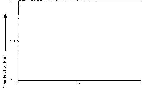
The ROC curve compares the classifiers’ performance across the entire range of class distributions and error costs. The ROC curve is given by TP rate and FP rate. ROC curve drawing algorithm use decision threshold values and construct the curve by sweeping it across from high to low. This gives rise to TP rate and FP rate at each threshold level which can intern be interpreted as points on the ROC curve. For more detail on ROC curve drawing algorithm one can refer to the work done by Hamel [35]. AUC provides a good measure of comparing the performances of ROC curves in particular to the cases where dominance of one curve is not fully established. More details can be found in Ling et. al. work [33]. In case of perfect predictions the AUC is 1 and if AUC is 0.5 the prediction is random.

The model performance through ROC curves for our classification models is shown in Fig. 2, Fig. 3 and Fig. 4. The X-axis represents False Positive Rate and Y-axis represents the True Positive Rate. For original randomized dataset, the average AUC value obtained are 0.995, 0.999 and 0.894 for J48, BayesNet and the LIBLINEAR classification models respectively. For the synthetically increased datasets, the corresponding average AUC values are 0.997, 1 and 0.907. Thus comparing the results in Table 2, Table 3, Table 4, Table 5 and AUC values, we can say BayesNet using Genetic search provides the best classifier. Nevertheless, J48 takes very less time in building the training model with a reasonably good model performance.

gives both high predictive accuracy and faster model building time. Therefore, we used the indirect method of building classification rules i.e. to extract rules from C4.5 classification model discussed in Section V. Rule induction from Quinlan’s famous C4.5 algorithm [24] is the conjunction of antecedents to arrive at a consequence. That is, if A, B and C are the test nodes encountered in the path from root to leaf node D, then the rule generated would be in conjunctive form such as “if A and B and C then D”. The approach for rule generation is as follows:

First we trained the C4.5 tree. Then from it we extracted initial set of rules by considering test conditions in each path as conjunctive rule antecedents and corresponding class labels as rule consequences. We extracted 21 such rules from the decision tree trained on our dataset. Then we remove those antecedents which can trivially be removed. For example, if there are two antecedents in the same rule, say t>x1 and t>x2 where t is the attribute and x1, x2 are the numeric attribute values such that x1>x2, then we accept the antecedent t>x1 and

VI.   A RULE INDUCTION ALGORITHM FOR

BOTNET TRAFFIC CLASSIFICATION

From analysis of results obtained from three classifiers in Section VI, it is apparent that Decision Tree (J48)

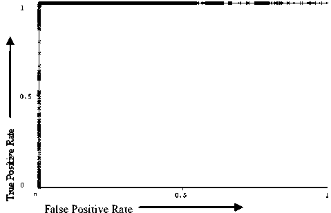
Figure 2: ROC curve for the BayesNet classification model (Class: P2Pbot)

False Positive Rate                          ►

Figure 3: ROC curve for the J48 classification model. (Class: P2Pbot)

False Positive Rate

Figure 4: ROC curve for the LIBLINEAR classification model. (Class: P2Pbot)

discard the other. Similarly, if antecedents were t

We computed Coverage and Accuracy for our initial set of C4.5 rules. Coverage is the fraction of records that satisfy antecedents of a rule, given by

Coverage = (|LHS|) / n (5)

And, accuracy is fraction of records covered by the rule that belong to the class on the RHS. It is given by

Accuracy = (|LHS ∩RHS|) / (|LHS|) (6)

Where n is the number of records in our dataset, |LHS| is the number of records that satisfies antecedent of a rule and |LHS ∩ RHS| is the number of records that satisfies the rule as a whole.

In our trained C4.5 tree, the attribute ‘response packet difference’ is the root followed by number of splitting on attributes ‘ratio of largest packet’ and ‘largest packet’. Only in one case ‘response packet difference’ and ‘response time difference’ is used for splitting dipper in the tree. The initial set of rule is generalized by removing antecedents not contributing to accuracy and coverage of its original rule. To do this, antecedents corresponding to test nodes higher up in the tree were removed first (initially the root node). Then the Coverage and accuracy values for remaining part of the rules containing antecedents corresponding to test nodes dipper down the tree were calculated. If the freshly calculated coverage and accuracy values were not worse than the original, we replaced the original rule with its new variant. This process was repeated until further generalization of the rules was not possible. Rules are then grouped according to their predicted classes and subjected to further polishing using Minimum Description Length (MDL) principle [36] so that rules that do not contribute to the accuracy of our rule based classifier are removed.

In our newly generated rule set, we are left with ten rules that predicted normal traffic and four rules for botnet traffic, down from fourteen and seven respectively for our initial rule set. One important observation of our newly generated optimized rule set is that there are seven rules out of fourteen which have flows classified based on “proportions of large packets transferred in a flow” and “packets carrying maximum payload” only. This is shown in Table 6. This led us to believe that some more rules of our new rule set can be modified to fall within mutually exclusive ranges of these two attribute values without / insignificant degradation of their corresponding coverage and accuracy values.

We applied heuristic method to create a variant of some of the existing rules of the remaining rule set. The procedure adopted to modify remaining part of the rule set is as follows: We created a list of test conditions that belongs to remaining rules in the rule-set. Then we weighted each test condition according to summation of coverage values of their participated rules. We grouped them according to attribute name and arranged it in decreasing order of their weight-age values in each group separately. Then we considered one rule at a time from the remaining pool and used heuristic to replace one of its antecedents For example, in case of the following rule that predicts Normal flow,

“If (Response packet difference ≤ 0.003) And (Ratio of largest packet ≤ 0.504274) And (Largest packet ≤ 0.0115) And (Largest packet > 0.0063) Then Class = Normal” we replaced the antecedent (Response packet difference ≤ 0.003) with (Ratio of largest packet > 0.142857). The new rule generated with this replacement has an accuracy and coverage of 100% and 1.68 % respectively. The corresponding figures for the rule before replacement were 99% and 1.15%. Table 7 shows new variant of four such rules. However, in three rules we need to retain antecedents on other two attributes for correct prediction. Those three rules are shown in Table 8.

Finding the best decision tree is NP-hard and all current decision tree algorithms are heuristic algorithms. Therefore, the decision tree structures would be different for different training sets. However, using our approach most of the rules can be converted in to ranges of packet carrying maximum payload and its proportions in a flow.

We have generated the rules from decision tree created on one data set and tested it on all the three data sets. We found that rules in Table 6 has a coverage of approximately 24%, rules in Table 7 has a coverage of approximately 76% and rules in Table 8 has a very negligible coverage. We also found that the rule based approach has produced better accuracy (Average Accuracy = 99.63 %) than the original decision trees in all the three test cases.

• VII. CONCLUSION AND FUTURE WORK

In this paper, we have proposed a methodology for detecting P2P botnets using Machine Learning techniques. We used

TABLE 6: Rules based on “ratio of largest packet” and “largest packet” only

Rule antecedents		Rule Consequence	Accuracy (%)
Ratio of Largest Packets	Largest Packet
> 0.504274	-	Normal	99.8
<= 0.142857	> 0.0457	Normal	99.3
<= 0.142857	<= 0.0083	Normal	100
<= 0.142857	> 0.0095 AND <= 0.0117	Normal	100
<= 0.142857	> 0.0118 AND <= 0.0365	Normal	97.7
> 0.00831 AND <= 0.142857	> 0.0365 AND <= 0.457	Normal	100
<= 0.142857	> 0.0117 AND <= 0.0118	P2Pbot	100

TABLE 7: Replaced antecedents in the new rules

Rule Antecedents			Rule Consequence	Accuracy (%) before replacement	Accuracy (%) after replacement
Replaced Antecedents	Replaced With	Unchanged Antecedents
(Response Packet Difference ≤ 0.003)	(Ratio of Largest Packet > 0.142857), (Ratio of Largest Packet <= 0.504274)	(Largest Packet > 0.0118)	Normal	99.5	99.7
(Response Packet Difference ≤ 0.003)	(Ratio of Largest Packet > 0.142857)	(Ratio of Largest Packet <= 0.504274), (Largest Packet > 0.0063), (Largest Packet <= 0.0115)	Normal	99	100
(Response Packet Difference ≤ 0.003)	(Ratio of Largest Packet > 0.142857)	(Ratio of Largest Packet <= 0.504274), (Largest Packet <= 0.0063)	P2Pbot	99.8	99.8
(Response Packet Difference ≤ 0.003)	(Ratio of Largest Packet > 0.142857)	(Ratio of Largest Packet <= 0.504274), (Largest Packet > 0.0115), (Largest Packet <= 0.0118)	P2Pbot	100	99.9

TABLE8: Unchanged rules

Rule Antecedents	Rule Consequence	Accuracy (%)
(Response Packet Difference > 0.003), (Ratio of Largest Packet <= 0.00831), (Largest Packet > 0.0365), (Largest Packet <= 0.0457), (Response Time Difference <= 0.01261)	Normal	100
(Response Packet Difference <= 0.003), (Ratio of Largest Packet <= 0.142857), (Largest Packet > 0.0083), (Largest Packet <= 0.0095), (Response Time Difference <= 0.01261)	Normal	100
(Response Packet Difference > 0.003), (Ratio of Largest Packet <= 0.142857), (Largest Packet > 0.0083), (Largest Packet <= 0.0095)	P2Pbot	100

Other classification algorithms such as J48 and LIBLINEAR are very fast. For example J48 took only 0.85 second to build model on our training data having a reasonably good predictive accuracy. Therefore, a noteworthy contribution of this research work is that we proposed a machine learning based framework for quick detection of P2P botnet traffic that has a high predictive accuracy. Our ROC curve analysis points to predictive accuracy of our classification models. However, we need to test our classification techniques in large-scale network set-ups.

Finally, we proposed a rule induction algorithm for P2P botnet traffic classification. We achieved better classification accuracy than decision tree classifier. We generated rules from traffic samples collected from Nugache botnet. However, same procedure can be adopted to generate rules for other P2P botnet traffic samples as well. Furthermore, our rule based approach can be a stepping stone for development of an unsupervised detection technique. Large number of botnet flows tends to exist within short intervals of proportions at which largest packets are transferred and also the size of the largest packet. Only when these two characteristic features failed to provide high predictive accuracy for a particular range of its values, the other two features were used.

Acknowledgment

We would like to thank Mohammad M. Masud, Department of Computer Science, University of Texas at Dallas for providing us the botnet dataset to carry out this research work.