An Empirical Method for Optimization of Counterpropagation Neural Network Classifier Design for Fabric Defect Inspection

Published Online August 2014 in MECS

Product quality assurance is treated as one of the most significant focuses in the industrial production. Product quality is severely lessened by defects. Failure to early defect detection incurs costs in terms of time, money and consumer satisfaction. So, early and accurate defect detection is an important aspect of quality control. Manual inspection is time consuming and the accuracy level is not good enough to meet the present demand of the highly competitive national and international market. The solution to the problems posed by manual inspection id automated, i.e. machine vision based defect inspection system. This is why, machine vision based defect inspection system is very challenging topic for research in various domains of industrial products, e.g. integrated circuits, printed circuit boards, ball grid arrays [1], ceramic tiles [2], sandpaper, castings, leather [3] and even cigarettes packaged in a tin container [4]. Likewise machine vision based fabric defect inspection system is a good thrust for the researchers of many countries. Automated fabric defect inspection systems mainly involve two challenging problems, namely defect detection and defect classification.

Automated fabric defect inspection systems are realtime applications. So they require real-time computation, which exceeds the capability of traditional computing. Neural networks (NNs) are suitable enough for real-time systems because of their parallel-processing capability. Moreover, NNs have strong capability to handle classification problems with good classification accuracy. They vary in network architecture as well as training or learning algorithm. There is a number of performance metrics of NN models. Classification accuracy, model complexity and training time are three of the most important performance metrics of NN models.

Counterpropagation neural networks (CPNs) can have good performance as classifiers. They can be employed in real-time systems. They are hybrid network, which are capable of handling complex classification problems with good classification accuracy [5-7]. Again, the number of computing units in a CPN model is low. This makes network topology simple, i.e. model complexity becomes low. Moreover, different types of learning algorithms are employed for each layer in a CPN, which results in short training time of the network [7, 8]. So a CPN appears to be a very good choice as a classifier in order to address the problem of fabric defect classification.

Although there have been some reports about the feasibility of neural network based classifier development for fabric defect classification, but there has been no reported work investigating interrelationship between design parameters and performance of NN based classifier. Concept demonstration alone is not sufficient to empower an application engineer to design optimum classifier. Therefore, this work not only focuses on the study of the feasibility of CPN model in the context of fabric defect classification, but also reports the findings of empirical investigation about the implications of CPN design parameters on the training and classification performance. In particular, we empirically discover the interrelationship between the performance metrics, accuracy and training time and the CPN design parameters, Kohonen learning constant (ηK), Grossberg learning constant (ηG) and model complexity (number of computing units in the hidden layer). Finally, we compare the performance of the CPN model with that of the classification models described in different articles.

The rest of the paper is organized as follows. Section II describes current state of solution to address the problem of fabric defect classification and Section III describes the design of CPN model. In Section IV, the defects and features set are presented describing our approach to solve the problem. Section V describes how we implement our CPN model and the results achieved after implementation. In Section VI, we have reviewed automated fabric defect classification results to develop an understanding of the merits of our CPN model. Finally, we give conclusion along with limitations and scope for future work in Section VII.

• II.   Literature Review

NNs have been deployed in order to solve the classification problem of different automated systems [915]. Likewise NNs have been involved in the research of automated fabric defect inspection system. Many efforts have been given for automated fabric defect inspection [8, 17-36]. Most of them have focused on defect detection, where few of them have focused on classification. NNs have been used as classifiers in a number of articles. Different learning algorithms have been used in order to train the NNs. None of them has performed a thorough investigation on finding an appropriate NN model. That means none  of them has performed a thorough investigation  on interrelationship between design parameters and performance of NN model.

Habib and Rokonuzzaman [17] have deployed CPN in order to classify four types of defects. Basically, they concentrated on feature selection rather than giving attention to the CPN model. They have not performed indepth investigation on interrelationship between design parameters and performance of CPN model.

Backpropagation learning algorithm has been used in [18], [19], [20], [21] and [22]. Habib and Rokonuzzaman [18] mainly focused on feature selection rather than focusing on the NN model. They have used four types of defects and two types of features. Saeidi et al. [19] have first performed off-line experiments and then performed on-line implementation. In both cases, they have used six types of defects. Karayiannis et al. [20] have used seven types of defect. They have used statistical texture features. Kuo and Lee [21] have used four types of defect. Mitropulos et al. [22] have used seven types of defects in their research. Detailed investigation on interrelationship between design parameters and performance of NN model has not been performed in any of these works discussed.

Resilient backpropagation learning algorithm has been used to train NN in [23] and [24]. They have worked with several types of defects considering two of them as major types and all other types of defects as a single major type. They have not reported anything detailed regarding the investigation of finding an appropriate NN model.

Shady et al. [25] have used learning vector quantization (LVQ) algorithm in order to train their NNs. They have used six types of defects. They have separately worked on both spatial and frequency domains for defect detection. Kumar [28] has used two NNs separately. The first one was trained by backpropagation algorithm. He has shown that the inspection system with this network is not cost-effective. So he has further used linear NN trained by least mean square error (LMS) algorithm. The inspection system with this NN is cost-effective. Karras et al. [30] have also separately used two NNs. They have trained one NN by backpropagation algorithm and the other one by Kohonen’s Self-Organizing Feature Maps (SOFM). Thorough investigation on interrelationship between design parameters and performance of NN model has not been reported in any of these reviewed works.

• III.    CPN Model

CPN is a hybrid network having two training phases: unsupervised learning and supervised learning. The unsupervised learning takes place between the input layer and hidden layer, and the supervised one takes place between the hidden layer and output layer. For our CPN, the unsupervised and supervised learning are Kohonen unsupervised and Grossberg supervised learning algorithms respectively.

• A.    Choice of Activation Function

The selection of an inappropriate activation function increases the complexities of the subsequent steps of CPN model design and makes the classification task difficult. On the contrary, the choice of an appropriate activation function smoothes out the difficulties lying in the subsequent steps of CPN model design and results in good performance.

• B.    Initialization of Weights

Each training phase in our CPN, i.e. Kohonen unsupervised learning and Grossberg supervised learning, begins with initial weight values that are randomly chosen. Large range of weight values may lead the training phases to take more number of training cycles.

• C.    Choice of Kohonen Learning Constant (η_K) and

Grossberg Learning Constant (ηG)

ηK and ηG are independent parameters, which determine how quickly learning being performed. Large values of ηK and ηG cause rapid learning, but there is a risk that the learning, i.e. search process, may oscillate. Again, small values of ηK lead to slow learning [6]. In fact, the right values of ηK and ηG depend on the nature of the classification problem of intended application such as fabric defects inspection system.

• D.    Reduction of Computing Units

Computation is too expensive with a large number of computing units. Again, training process does not converge with too small number of computing units. That means the NN will not be powerful enough to solve the classification problem with too small number of computing units. In fact, the right size of NN depends on the specific classification problem that is being solved using NN.

(c)                                              (d)

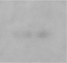
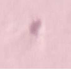
Fig. 1. Different types of defect occurred in knitted fabrics. (a) Color yarn. (b) Hole. (c) Missing yarn. (d) Spot.

IV. Approach and Methodology

We are to address the problem of empirically discovering the interrelationship between performance metrics, accuracy and training time, and the network design parameters, Kohonen learning constant ( η K ), Grossberg learning constant ( η G ) and model complexity (number of computing units in the hidden layer). We want to maximize accuracy and minimize training time. Both accuracy and training time depend on model complexity, Kohonen learning constant and Grossberg learning constant. If accuracy, training time, model complexity, the number of computing units in the input, hidden and output layer are represented by A , T , C M , N I , N H and H O respectively, then

B. An Appropriate Feature Set

An appropriate feature set is selected for classifying the defects. All of these four features can be found in detail in [17] for readers.

A = f l (C M , П к , n )

V. Implementation

We start with inspection images of knitted fabric of size 512×512 pixels, which are converted into a grayscale image. In order to smooth these images and remove noises, they are filtered by 7×7 low-pass filter convolution mask. Then gray-scale histograms of the images are formed. Two threshold values θ L and θ H are calculated from each of these histograms using histogram peak technique [37]. Using the two threshold values θ L and θ_H , images with pixels P(x, y) are converted to binary images with pixels I_B(x, y) , where

and T = f 2⁽ C M , П к , П ), where C M = ( N I , N H , N O )

Jl,   if O l <  P ( x, y ) <  9 h

I ( x, y ) = <

10, otherwise

.

So the optimization problem is defined as follows: maximizef i ( c m , П к , 9 g ) and minimize f_г(С_м, q _K , 9 g )

subject to Nj = 4

Nh ^ 6

No = 6

0 < 9k < 1

0 < 9g < 1

These binary images contain objects (defects) if any exists, background (defect-free fabric), and some noises. These noises are smaller than the minimum defect wanted to detect. In our approach, we want to detect a defect of minimum size 3mm×1mm. So, any object smaller than the minimum-defect size in pixels is eliminated from the binary images. If the minimum defect size in pixels is θ MD and an object with pixels Obj(x, y) is of size N obj pixels, then

A. Defect Types

In this article, we have worked with four defect types, which frequently occur in knitted fabrics, namely color yarn, hole, missing yarn (horizontal and vertical) and spot. All of the defects are shown in Figure 1.

Obj ( x , y ) = 11-   -fN obj ^ ^O md

10, otherwise

.

(a)

(b)

Then a number of features of defects are calculated, which forms feature vectors corresponding to defects present in images.

The classification step consists of the tasks of finding proper CPN model from a number of CPN models. Building a CPN model involves two phases, namely training phase and testing phase. For this purpose, one hundred color images of defective and defect-free knitted fabrics of seven colors are acquired. So, the number of calculated features or input vectors is 100. That means our sample consists of 100 feature vectors. Table 1 shows the frequency of each defect and defect-free class in our sample of 100 images.

Table 1. Frequency of Each Defect and Defect-Free Class

No.	Class	Frequency
1	Color Yarn	6
2	Vertical Missing Yarn	16
3	Horizontal Missing Yarn	16
4	Hole	11
5	Spot	18
6	Defect-Free	33
	Total	100

The features provided by the feature extractor are of values of different ranges, which causes imbalance among the differences of feature values of different defect types and makes the training phase difficult. The scaling, shown in (3), (4), (5), and (6), of the features is made in order to have proper balance among the differences of feature values of defect types. If H^/_DW , W^/ DW , R^/ H/W and N^/ DR represent the scaled values of the features provided by the feature extractor H DW , W DW , R H/W , and N DR , respectively, then

HDW = HDW X100.(3)

W

Wdw = 1D2" x W0.(4)

RH/ W = 100 X RH/ W .

Ndr = 500(Ndr - 1)x 10999 .(6)

We split all feature vectors into two parts. One part consisting of 53 feature vectors is for both testing and training the CPN model and the other part consisting of the rest of the feature vectors is for testing only. The target values are set to 1 and 0s for the corresponding class and the rest of the classes, respectively. That means if a feature vector is presented to the CPN model during training, the corresponding computing unit in the output layer of the corresponding class of the feature vector is assumed to fire 1 and all other units in the output layer are assumed to fire 0. The CPN model is trained with maximum number of training cycle 106, maximum amount of training time 1 hour and maximum tolerable error less than 10-3. That means training continues until 106 training cycles and 1 hour is elapsed and error less than 10-3 is found. After the training phase is completed, the CPN model is tested with all the feature vectors of the both parts. Then all feature vectors are again split into two parts. The first fifty percent of the part for training comes from the previous part for training and the rest fifty percent comes from the previous part for only testing. All other feature vectors form the new part for only testing. The CPN model is trained with these new parts and then is tested. In this way, for a specific combination of CPN design parameters, the model is trained and tested from 3 to 5 times in total. We take the results which mostly occur. If the results are uni-modal, we take the results that are the closest to their averages.

In accordance with CPN architecture, we use three-layer feedforward NN for our model assuming that input layer contributes one layer. We started with a large CPN that has 4 computing units in the input layer, 48 computing units in the hidden layer and 6 computing units in the output layer (since we have six different classes according to Table 1). We describe the entire training, where the number of feature is 4, in detail in the following parts of this section, i.e. Section V.

• A.    Choice of Activation Function

For our CPN, the unsupervised and supervised learning are the Kohonen and Grossberg learning respectively. For Kohonen unsupervised learning, we implement a piecewise activation function, which is defined as follows:

f ⁽ x ) =

f 1,

0,

if x is the closest according to the closeness criterion otherwise

Here in (7), the closeness criterion is distance-based, i.e. the Euclidean distance between feature vectors and the weights of each computing unit in the hidden layer. For Grossberg supervised learning, we implement a linear activation function, which is defined as follows:

f (x ) = x .

• B.    Initialization of Weights

In our implementation, we randomly choose initial weight values of small range, i.e. between -1.0 and 1.0 exclusive, rather than large range, e.g. between -103 and 103 exclusive for each of the two training phases in our CPN.

• C.    Choice of Kohonen Learning Constant (η K ) and Grossberg Learning Constant (η G )

We first train as well as test the CPN for η_K = 0.01 and η_G = 0.01. We gradually increase the value of η_K , and train as well as test the NN for that value of η K keeping the value of η G fixed. Obtained results are shown in Table 2. We find that the error function (sum of squared error, E ) is tolerable, i.e. less than 10^-3, and the accuracy is maximum, i.e. 100%, for 0.2 ≤ η K ≤ 0.35. We choose 0.2 as the value of η K since the number of elapsed training cycle is the minimum, i.e. 305 at 0.2 for 0.2 ≤ η_K ≤ 0.35.

Likewise we first train as well as test the CPN for η G = 0.01 and η K = 0.2. We gradually increase the value of η G , and train as well as test the NN for that value of η G keeping the value of η K fixed. The results achieved are shown in Table 3. We find that E is tolerable and the accuracy is the maximum for 0.01 ≤ η G ≤ 0.8. Although the number of elapsed training cycle is the minimum, i.e. 2 for η_G = 0.99, we choose 0.8 as the value of η_G since E is the minimum, i.e. 1.604471 × 10^-10 for η G = 0.8.

The classifier design objective of an application engineer is to peak such values of Kohonen and Grossberg learning constants which require minimum training time and produces maximum classification accuracy. From this investigation, it appears that the

Kohonen learning constant having value in between 0.2   produces the highest accuracy. minimum training time and 0.35 and Grossberg learning constant having value in   and produces the highest accuracy.

between 0.1 and 0.8 require minimum training time and

Table 2. Results of Tuning Kohonen Learning Constant η K

Network Topology (Number of Computing Units)			Kohonen Learning Constant ( η K )	Grossberg Learning Constant ( η G )	Error Function (E)	Number of Elapsed Training Cycle	Accuracy
Input Layer	Hidden Layer	Output Layer
4	48	6	0.01	0.01	5.386981	81	83%
			0.05		6.839689	41	81%
			0.1		2.886601	1754	89%
			0.15		2.886601	1777	89%
			0.2		9.803619 × 10-4	305	100%
			0.25		9.822536 × 10-4	322	100%
			0.3		9.852246 × 10-4	351	100%
			0.35		9.879542 × 10-4	362	100%
			0.4		1.855984	1806	92%
			0.45		1.875984	1846	92%

Table 3. Results of Tuning Grossberg Learning Constant η G

Network Size (No. of Computing Units)			Kohonen Learning Constant ( η K )	Grossberg Learning Constant ( η G )	Error Function (E)	Number of Elapsed Training Cycle	Accuracy
Input Layer	Hidden Layer	Output Layer
4	48	6	0.2	0.01	9.824014 × 10-4	304	100%
				0.1	9.742609 × 10-4	36	100%
				0.2	6.035657 × 10-4	31	100%
				0.3	3.962778 × 10-4	30	100%
				0.4	6.430443 × 10-6	30	100%
				0.5	1.102199 × 10-4	29	100%
				0.6	4.222798 × 10-6	29	100%
				0.7	4.762689 × 10-8	29	100%
				0.8	1.604471 × 10-10	29	100%
				0.9	8.264628 × 10-5	17	94.85%
				0.99	9.314982 × 10-4	2	65.98%

Table 4. Results of Reducing Computing Units in Hidden Layer

Network Topology (No. of Computing Units)			Kohonen Learning Constant ( η K )	Grossberg Learning Constant ( η G )	Error Function (E)	Number of Elapsed Training Cycle	Accuracy
Input Layer	Hidden Layer	Output Layer
4	48	6	0.2	0.8	1.268166 × 10-10	29	100%
	45				0.08264256	6	93.81%
	42				1.690904 × 10-10	29	100%
	39				0.08264299	6	93.81%
	36				1.766581 × 10-10	29	100%
	33				0.08264259	6	93.81%
	30				2.483729 × 10-10	29	100%
	27				0.08264286	6	93.81%
	24				1.628943 × 10-10	29	100%
	21				0.06835751	6	93.81%
	18				0.001111822	17	94.85%
	15				0.06832235	6	93.81%
	12				0.08264268	6	93.81%

• D.    Reduction of Computing Units

One approach to find the right size of NN is to start training and testing with a large NN. Then some computing units and their associated incoming and outgoing edges are eliminated, and the NN is retrained and retested. This procedure continues until the network performance reaches an unacceptable level [38, 39].

Following the approach, we first train as well as test a large CPN, which has 4 computing units in the input layer, 48 computing units in the hidden layer and 6 computing units in the output layer. Then we successively eliminate 3 computing units in the hidden layer, and train as well as test the reduced CPN. We carry on the procedure until the network performance reaches an unacceptable level. The achieved results are shown in Table 4. We find that there are fluctuations in error function (E) and the accuracy as the number of computing units in the hidden layer decreases from 48. E is tolerable, i.e. less than 10-3 and the accuracy is the maximum, i.e. 100%, for multiple values of the number of computing units in the hidden layer. We also find that training finishes at the minimum number of training cycle, i.e. 6 for multiple values of the number of computing units in the hidden layer.

The classifier design objective of an application engineer is to choose such network topology that requires minimum training time and produces maximum classification accuracy. From this investigation, it appears that the network topology with 6 i (4 ≤ i ≤ 8) computing units in hidden layer requires much training time and produces the highest accuracy and the network topology with 3+6 i (3 ≤ i ≤ 7) computing units in hidden layer requires minimum training time and produces less accuracy. All of these investigations are summarized in Table 5.

Table 5. Summary of the results of all investigations

Design Parameter	Optimum Band	Number of Elapsed Training Cycle	Accuracy
Kohonen learning constant ( η K )	0.2 – 0.35	305 – 362	100%
Grossberg learning constant ( η G )	0.1 – 0.8	36 – 29	100%
Network topology (no. of computing units)	4-6 i -6 (4 ≤ i ≤ 8)	29	100%

We find that the minimum number of computing units in hidden layer, for which accuracy is highest, is 24. Where the number of classes is 6 only, 24 seems to be large enough. So, we rescale the feature, the number of defective regions ( N DR ), to accentuate the differences between the number of defective regions and all other features so that the performance can be improved.

• E.    Introduction of Rescaling

W If N^// DR represents the rescaled value of N^/ DR in (6), then N^//_DR is defined by the following equation:

N DR = 10 X N dr .                             (9)

We start training and testing a CPN, which has 24 computing units in the hidden layer, with the rescaled feature or input vectors. Then we gradually eliminate some computing units in the hidden layer, and train as well as test the reduced CPN. We carry on the procedure until the network performance reaches an unacceptable level. The results achieved are shown in Table 6. We find that the accuracy is tolerable, i.e. less than 10-3 and the accuracy is the maximum, i.e. 98.97% as long as the number of computing units in the hidden layer is greater than 6. Moreover, the number of elapsed training cycle is only 6 as long as the number of computing units in the hidden layer is greater than 6 too.

Table 6. Results of Reducing Computing Units in Hidden Layer after Rescaling

Network Topology (No. of Computing Units)			Kohonen Learning Constant ( η K )	Grossberg Learning Constant ( η G )	Error Function (E)	Number of Elapsed Training Cycle	Accuracy
Input Layer	Hidden Layer	Output Layer
4	24	6	0.2	0.8	2.627666 × 10-6	6	98.97%
	21				2.640732 × 10-6	6	98.97%
	18				2.653941 × 10-6	6	98.97%
	15				2.677102 × 10-6	6	98.97%
	12				2.709638 × 10-6	6	98.97%
	9				2.66666 × 10-6	6	98.97%
	8				2.66666 × 10-6	6	98.97%
	7				2.66666 × 10-6	6	98.97%
	6				0.1498665	11	92.78%

• VI.    Comparative Performance Analysis

In order to assess merits of our implemented CPN model for classifying fabric defects, let’s compare some recently reported relevant research results. It is to be noted that assumptions taken by researchers in collecting samples and reporting results of their research activities in processing those samples will have serious implications on our attempt of comparative performance evaluation. The review of literature reveals that most of research reports are limited to the demonstration of concepts of machine vision based approach to fabric defect classification without the support of adequate numerical results and their comparison with similar works. Moreover, the absence of use of common database of samples of fabric defects makes it difficult to have a fair comparison of merits of different algorithms. Similar observation has been reported by Kumar in a comprehensive survey [16].

Kumar has also mentioned in his conclusion that although last few years have shown some encouraging trends in fabric defect inspection research, systematic/comparative performance evaluation based on realistic assumptions is not sufficient. Despite such limitations, we have made an attempt to review numerical results related to fabric defect classification to assess comparative merits of our work.

A number of learning algorithms have been used in order to train the NNs. Backpropagation learning algorithm has been used in [18], [19], [20], [21] and [22]. Habib and Rokonuzzaman [18] have worked with knitted fabrics. Their sample consisted of 100 images. They have used a three-layer feedforward NN, which had 4, 12 and 6 computing units in the input, hidden and output layers respectively. It took 88811 cycles for the NN to be trained. A 100%-accuracy has been found. Although the accuracy and model complexity (number of computing units) have been good and medium respectively, the training time has been long. Saeidi et al. [19] have worked with knitted fabrics. They have first performed off-line experiments and then performed on-line implementation. In case of off-line experiments, the sample size was 140. They have employed a three-layer feedforward NN, which had 15, 8 and 7 computing units in the input, hidden and output layers, respectively. It took 7350 epochs for the NN to be trained. An accuracy of 78.4% has been achieved. The model complexity has been modest. Moreover, the training time has been long and the accuracy has been poor. In case of on-line implementation, the sample size was 8485. An accuracy of 96.57% has been achieved by employing a feedforward NN. The accuracy has been good although the model complexity and training time have not been mentioned. Karayiannis et al. [20] have worked with web textile fabrics. They have used a three-layer NN, which had 13, 5 and 8 computing units in the input, hidden and output layers, respectively. A sample of size 400 was used. A 94%-accuracy has been achieved. Although the accuracy and model complexity have been good and small, respectively, nothing has been mentioned about the training time.

Kuo and Lee [21] have used plain white fabrics and have got accuracy varying from 95% to 100%. The accuracy has been modest. Moreover, the model complexity and training time have not been reported. Mitropulos et al. [22] have used web textile fabrics for their work. They have used a three-layer NN, which had 4, 5 and 8 computing units in the input, hidden and output layers, respectively. They have got an accuracy of 91%, where the sample size was 400. The accuracy has been modest although the model complexity has been small. Nothing has been mentioned about the training time.

Resilient backpropagation learning algorithm has been used in [23] and [24]. Islam et al. [23] have used a fully connected four-layer NN, which contained 3, 40, 4, and 4 computing units in the input, first hidden, second hidden and output layers, respectively. They have worked with a sample of over 200 images. They have got an accuracy of 77%. The accuracy has been poor and the model complexity has been large. Moreover, the training time has not been given. Islam et al. [24] have employed a fully connected three-layer NN, which had 3, 44 and 4 computing units in the input, hidden and output layers, respectively. 220 images have been used as sample. An accuracy of 76.5% has been achieved. The accuracy and model complexity have been poor and large, respectively. Moreover, nothing has been mentioned about the training time.

Habib and Rokonuzzaman [17] have worked with CPN. Their sample consisted of 100 images of knitted fabrics. Their CPN had 4, 12 and 6 computing units in the input, hidden and output layers respectively. About 200 cycles was taken for the training of CPN. An accuracy of 100% has been achieved. Although the accuracy and training time have been good, the model complexity (number of computing units) has been too long in the context of CPN.

Shady et al. [25] have separately worked on both spatial and frequency domains in order to extract features from images of knitted fabric. They have used the LVQ algorithm in order to train the NNs for both domains. A sample of 205 images was used. In case of spatial domain, they employed a two-layer NN, which contained 7 computing units in the input layer and same number of units in the output layer. They achieved a 90.21%-accuracy. The accuracy has been modest although the model complexity has been small. Moreover, the training time has not been given. In case of frequency domain, they employed a two-layer NN, which had 6 and 7 computing units in the input and output layers, respectively. An accuracy of 91.9% has been achieved. Although the model complexity has been small, the accuracy has been modest. Moreover, nothing has been mentioned about the training time.

Table 7 shows the comparison of our CPN model and others’ NN models. For our CPN model as shown in Table 7, we consider the best result found after entire implementation.

Kumar [16] has found that more than 95% accuracy appears to be industry benchmark. In that survey, it has been reported by Kumar in reviewing 150 articles that a quantitative comparison between the various defect detection schemes is difficult as the performance of each of these schemes have been assessed/reported on the fabric test images with varying resolution, background texture and defects.

With respect to such observation, our obtained accuracy of more than 98% appears to be quite good. Moreover, our model complexity (4, 7 and 6 computing units in the input, hidden and output layer respectively)

has been small and training time short (6 cycles). As we have mentioned earlier, due to the lack of uniformity in the image data set, performance evaluation and the nature of intended application, it is not prudent to explicitly compare merits of our approach with other works. Therefore, it may not be unfair to claim that our implemented CPN model have enough potential to classify fabric defects with very good accuracy.

Table 7. Results of the Comparison of CPN Model We Implemented and Others Implemented