An Enhanced Adaptive B-spline Smoothing Approach for UAV Path Planning

Unmanned Aerial Vehicles (UAVs) are now essential for various uses, such as autonomous navigation, aerial photography, urban monitoring, and disaster response. Advanced path planning algorithms that handle dynamic obstacle avoidance, collision prevention, and smooth trajectory execution are becoming increasingly necessary as UAV use increases in complicated situations like metropolitan regions and disaster zones. Notably, abrupt changes in trajectory can adversely impact vehicle stability and increase energy consumption, making path smoothing a crucial focus of research and development in UAV operations [1,2].

In recent years, UAV path planning has evolved into a multifaceted discipline that seeks to generate collision-free, dynamically feasible trajectories from an initial position to a designated goal. Classical formulations often regard path planning as a two-step process: first, finding a sequence of waypoints that avoids obstacles, and second, refining that waypoint sequence into a smooth, executable trajectory. Graph-based methods (e.g., A* and D*) discretize the environment into nodes and edges, guaranteeing optimality under certain metrics but potentially yielding jagged, piecewise-linear routes that can impose high control effort on the UAV. Sampling-based approaches (e.g., RRT and PRM) probabilistically explore the configuration space, producing feasible paths more rapidly in high-dimensional or partially known terrains, yet still require a postprocessing step to eliminate sharp turns and ensure dynamic compliance. Potentialfield methods treat obstacles and goals as repulsive and attractive forces, respectively, offering smooth vector fields but often suffering from local minima. Regardless of the underlying planner, the raw output must be smoothed or reparametrized to satisfy the vehicle’s kinematic and aerodynamic constraints—ensuring that velocity, acceleration, and curvature remain within allowable bounds. In practical applications such as urban inspection or disaster relief, real-time updates to both obstacle information and mission objectives further complicate path planning, demanding algorithms that balance computational speed, trajectory optimality, and robustness to environmental uncertainty.

UAV guidance is conventionally decomposed into two hierarchical stages. First, a global planner (e.g., A*, D*, RRT*) delivers a course, collision-free poly-line that guarantees obstacle clearance but pays little attention to vehicle dynamics. Second, a local trajectory generator refines this route into a time-parameterized curve whose curvature, velocity and jerk remain within the airframe’s flight envelope [3]. The effectiveness of this smoothing stage has a direct impact on tracking accuracy, control effort and energy consumption, particularly for small multirotor platforms whose high power-to-weight ratio magnifies the penalties associated with aggressive steering commands.

B-Splines, comprise a family of piece-wise polynomial basis functions defined over a non-decreasing knot vector that partitions the parameter domain [4]. Their compact support across at most k+1 knot spans endows them with the celebrated local-modification property: altering a single control point influences the curve only in its immediate neighborhood. For cubic B-Splines (k=3) this yields C2 continuity, ensuring smooth acceleration profiles without the oscillatory artefacts often observed in high-order global polynomials.

Among the various path-smoothing techniques, B-Splines (basis splines) have emerged as a powerful mathematical tool for optimizing UAV trajectories [5,6]. They are piecewise polynomial functions that provide local control and smoothness, allowing UAVs to navigate static and dynamic environments efficiently [7,8]. Researchers have significantly improved trajectory optimization, collision avoidance, and real-time path changes by combining B-Splines with hybrid path planning methods. Methods like gradient-based B-Spline trajectory optimization, which integrates real-time vision systems for dynamic obstacle tracking, further demonstrate the potential of B-Splines to improve UAV navigation tactics in uncertain environments [9,10].

The convex-hull property of B-splines keeps the generated path close to its control polygon, facilitating conservative yet efficient collision-checking, while their analytic derivatives simplify curvature and acceleration enforcement. Because both control-point positions and knot locations constitute low-dimensional decision variables, B-Spline trajectories can be optimized with evolutionary or gradient-based solvers under multi-objective criteria that simultaneously consider path length, dynamic feasibility and risk exposure. These characteristics explain the growing adoption of B-Splines in aerial robotics, where trajectories must satisfy not only geometric constraints but also stringent limits on angular rates, load factors and energy budget.

Practical applications of B-Spline smoothed trajectories can be found in a variety of fields, including search and rescue missions, aerial photography, and emergency medical delivery. In all of these cases, accurate and stable flight paths are critical to mission success [11]. Using B-Spline optimization techniques has been shown to improve energy efficiency, cut projected path lengths, and drastically reduce trajectory corners [12]. Nevertheless, several difficulties still exist despite these developments. Balancing computational efficiency with adaptability in real-time scenarios, optimizing path planning for both static and dynamic obstacles, and addressing trade-offs between competing optimization objectives (e.g., smoothness, path length) continue to be active areas of research [2, 11].

Additionally, multi-objective optimization in UAV path planning is a topic of ongoing discussion, as researchers try to balance a number of factors, including environmental constraints, flight stability, and energy consumption [13,14]. As UAV technology evolves, incorporating machine learning and advanced data processing techniques is expected to enhance path smoothing methodologies further, offering more adaptive and intelligent UAV trajectory planning solutions [15,2].

Recent advancements in UAV path planning increasingly leverage machine learning (ML) and deep learning techniques, such as deep reinforcement learning for end-to-end policy generation, or supervised/imitation learning for mimicking expert trajectories [16,17]. These methods excel in complex, dynamic environments by learning adaptive behaviors from data [18]. However, challenges persist regarding the formal safety guarantees, interpretability, explicit enforcement of C2 continuity or precise dynamic constraints, and the substantial data and training requirements often associated with machine learning approaches [19]. While powerful, their outputs may necessitate additional postprocessing to meet the stringent smoothness and feasibility criteria critical for stable UAV flight.

Table 1. Comparison of major track smoothing methods

Method	Pros	Cons
Filtering & Kalman	Good for moderate/mild maneuvers, can handle sensor noise well	Performance degrades with high-agility or abrupt maneuvers, requires careful tuning of process/noise models
Polynomial-Based (High-Order)	Straightforward to implement, can approximate smooth functions over intervals	Susceptible to Runge phenomenon (oscillations at boundaries), increasing order leads to higher sensitivity and complexity
B-Spline-Based	Local control (changes in control points/knot vector affect only portions of the curve), lower polynomial degree leads to smoother velocity	Requires careful knot selection
B-Spline with GA Optimization	Automates node (knot) selection, can adapt to complex trajectories	GA might be computationally more expensive; fitness function must be tuned to specific UAV/target dynamics

Table 1 provides a comprehensive comparison of the major track‐smoothing methods discussed above, highlighting each approach’s principal advantages and limitations.

In contrast, parametric curve methods like B-Splines, which form the basis of this work, offer inherent mathematical properties facilitating direct control over trajectory smoothness, curvature, and dynamic constraint satisfaction. The proposed enhanced adaptive B-Spline method builds upon this robust foundation, aiming to optimize these characteristics explicitly. While some advanced optimization algorithms like metaheuristics [20] are also employed in path planning, B-Splines provide a unique combination of local control and inherent smoothness. Our approach focuses on refining a mathematically transparent framework valuable for applications demanding verifiable path properties and predictable behavior, distinguishing it from primarily data-driven techniques and offering a complementary path that could integrate with ML for higher-level tasks in hybrid systems.

Recent research has put much effort into creating a UAV flight path that is responsive to flight dynamics and stays smooth. For instance, clustering techniques are used in [21] to locate a hover point, which guides the drone's subsequent movements. Fast, linear transitions between hover locations are made possible by different research that simultaneously optimizes the trajectory and speed, as described in [22]. Beyond UAV-centric examples, smoothing strategies have been examined for various robotic platforms. These include an improved ant colony algorithm for mobile robot navigation [23], an adaptive forward-looking pose interpolation algorithm for multi-segment path transitions [24], and continuous B-Spline-based smoothing for trolley robot paths [25]. Together, these studies reinforce the growing consensus that smoothing—especially via B-Spline-based approaches—plays a pivotal role in refining raw or partially planned trajectories for reliable, real-time deployment. Figure 1 compares polynomial interpolation and B-Spline fitting on a representative data set.

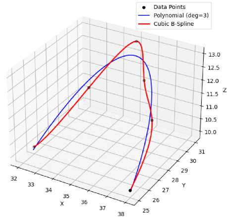
Fig.1. Polynomial vs. B-spline curves

Despite their merits, existing B-Spline methods may not be directly applicable or sufficiently robust for high-precision UAV track smoothing when strong constraints on flight dynamics, curvature, and acceleration come into play. Therefore, the present work proposes an enhanced cubic B-Spline smoothing method augmented with an adaptive knot selection mechanism and a carefully tailored fitness function that aligns with UAV maneuverability needs. By combining the strengths of B-Spline interpolation (convexity, local invariance, and low-degree polynomials) with a specialized genetic algorithm for node-vector refinement, the approach aims to improve the fidelity and safety of UAV trajectory data significantly.

2.    Problem Formulation

Effective track smoothing for aircraft or unmanned aerial vehicle (UAV) navigation can be formulated as an optimization problem, wherein a parametric curve must approximate a sequence of observed or measured waypoints under strict geometric and dynamic constraints. This section details the core mathematical and conceptual method underlying such a formulation, explicating the decision variables, objective functions, and constraints that guide the smoothing process.

• 2.1.    Overview of the Track Smoothing Task

Let {p0,p1, ■■■ ,Рц} denote a sequence of raw track points in either two- or three-dimensional space ((pi £ Rd) (d £ {2,3})) . These points often exhibit irregularities due to sensor noise, momentary measurement dropouts, or abrupt maneuvers. The goal of track smoothing is to construct a continuous, differentiable curve (C(u)) that passes near these points while adhering to physical and operational constraints.

• •    Data Fidelity: the smoothed curve should deviate minimally from the raw track data to preserve essential flight details.

• •    Dynamical Feasibility: the curve must obey kinematic and dynamic limits—most notably, maximum velocity, acceleration, and curvature—so that the aircraft or UAV can feasibly follow it in real flight.

• •    Computational Efficiency: the approach must be efficiently solvable for real-time or near real-time applications, particularly when dealing with high-dimensional or rapidly changing mission scenarios.

• 2.2.    B-spline Representation

A common choice for smooth trajectory generation involves B-Spline curves of fixed degree k. In the cubic case (k = 3) , each coordinate of the trajectory is represented by:

C(u) = ^m=0  dtNt^u),  ^Umin ^ ^U ^ ^Umax                            (1)

where:

• •    {d₀,..., d_m} are the control points in (R^d).

• •    -Мцк(и) are B-Spline basis functions of degree k.

• •     {u₀, U1, ..., U_m+fc+1} is the knot vector, partitioning the parameter domain [u_min, U_max] .

The smoothness of a B-Spline curve stems from the properties of these basis functions: they guarantee continuity up to the (k — 1) -th derivative across knot boundaries. For UAV track smoothing, cubic B-Splines typically offer an advantageous balance between computational demand and curvature continuity.

Figure 2 shows a simple example of a cubic B-Spline built from five control points. In the diagram, the control points are marked by blue circles, which are joined by dashed blue lines to form the control polygon. The red curve overlaying these points is the cubic B-Spline itself. Although the spline does not pass exactly through every control point, its shape is governed by their collective arrangement. Importantly, the entire red spline remains inside the convex hull of the blue control polygon, meaning that no portion of the curve escapes the “envelope” defined by the control points. This convex-hull property ensures that the curve’s geometry is predictable and makes it easier to reason about obstacle clearance in the UAV’s flight path.

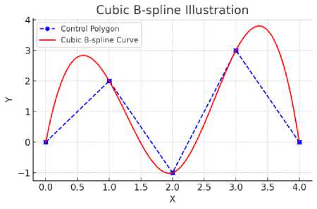
Fig.2. B-spline illustration

B-Spline curves offer local control, meaning that adjusting a specific control point affects the curve only in its immediate vicinity rather than causing large-scale deformations. Additionally, they remain within the convex hull of their control polygon and exhibit continuous first and second derivatives, which is beneficial for many real-world applications that require smooth transitions in velocity and acceleration. However, selecting the number and placement of knots (the node vector) can be challenging. An underspecified knot vector may oversimplify the trajectory, while an overly dense one increases complexity and can lead to overfitting.

When employing B-Splines, there are two sets of primary decision variables:

• •    Control Points D = {d ₀ ,..., d_m} . These determine the overall shape and position of the smooth curve. They may be obtained via direct fitting (e.g., least-squares) or optimization (e.g., genetic algorithms).

• •    Knot Vector^ = {u₀, U1, ..., U _m+fc+1 }. The node vector sets the parameter breakpoints that define how localized segments of the curve combine. Optimizing U can significantly enhance the curve’s adaptability to local features in the trajectory.

• 2.3.    Constraints for UAV Flight

In realistic flight scenarios, the smoothed trajectory must satisfy strict physical and operational constraints. First, the curvature constraint ensures that turns do not exceed the platform’s aerodynamic or structural limits.

к(С(и)) = ^^SjH <  _к                              (2)

^{v       J}        Це' (и)Ц³

Next, the velocity and acceleration bounds reflect the maximum speed and acceleration that the aircraft or UAV’s propulsion and control surfaces can support without jeopardizing safety or stability.

Цс ' MI <  ^max, Цс "  MI <  ^max                                (3)

In environments containing known obstacles, the curve С(u) must remain in free space. For cases requiring a safety margin, an enlarged “buffer zone” around each obstacle can be used to offset the smoothed path away from hazardous regions.

Finally, certain missions impose boundary conditions, such as fixed velocity or heading at the start or end point; these conditions must be respected throughout the smoothing or fitting process.

• 2.4.    Objective Function

Given that track smoothing aims to satisfy multiple criteria—fidelity to the raw trajectory, compliance with flight constraints, and minimization of abrupt maneuvers—an aggregate cost function can be formulated.

J(D, U = wi ^ _lata (C) + w ₂ ^ _curv (C) + w ₃ ^ _dyn (C) + w₄^ _en (C) + w ₅ ^ _mot(U)              (4)

where

• •    ^ ia _t a(C): Data Fidelity. This term measures how closely the smoothed B-Spline curve C(u) adheres to the

initial sequence of raw track points {p_t} . A common implementation is the sum of squared Euclidean distances between each raw point p_t and its closest corresponding point on the curve C (u) . Minimizing this term ensures that the smoothed path does not excessively deviate from the intended route defined by the global planner or sensor measurements, preserving essential flight details.

• •    ^c _Urv (C): Curvature Penalty. This component penalizes excessive curvature along the trajectory, promoting

smoother turns and reducing mechanical stress on the UAV. It is typically calculated by integrating the square of the curvature к(С(и)) along the path. This encourages trajectories that are well within the UAV's maneuverability limits, contributing to flight stability and reducing wear.

• •    ^ _dyn (C): Dynamic Feasibility Penalty. This term addresses adherence to the UAV’s flight envelope concerning

velocity and acceleration. Similar to the curvature penalty, it can be formulated to penalize deviations from desired operational ranges or violations of soft limits for velocity magnitude ЦС'(и)Ц  and acceleration magnitude ЦС (и)Ц.

• •    ^ ien (C) : Path Length. This term directly measures the total length of the B-Spline curve C(u) . Minimizing path

length is often desirable for energy efficiency and mission time reduction, provided it does not compromise safety or smoothness.

• •    ^ i <_not (U): Knot Distribution Regularization. This term aims to promote a well-behaved knot vector U. It can

penalize overly dense knot clusters, which might lead to overfitting or increased computational complexity, or excessively sparse distributions that might underrepresent critical path features. For instance, it could penalize large variations in knot spacing or deviations from a desired average knot density. This helps in achieving a balanced knot distribution that adapts to trajectory complexity without unnecessary complexity.

The non-negative scalar weights w1, w₂, w₃,w₄, w ₅ are crucial for tailoring the objective function to specific mission requirements and UAV characteristics. For example, in a surveillance mission where path smoothness and minimal deviation from a pre-planned route are critical for sensor stability, w1 (data fidelity) and w ₂ (curvature) might be assigned higher values. Conversely, for a rapid search-and-rescue mission, w ₃ (path length) might receive greater emphasis to minimize flight time, while still maintaining sufficient smoothness and dynamic feasibility through w ₄ and w ₅ . The selection of these weights is typically an iterative process, often guided by empirical evaluation, simulation, or domain expertise to achieve the desired balance between competing objectives. This weighted sum approach transforms the multiobjective optimization problem into a single-objective one, suitable for optimization algorithms.

By explicitly incorporating kinematic, dynamic, and environmental factors into the smoothing process, the resulting path remains feasible for real-world UAV operations. This approach effectively meets the multifaceted demands of modern air navigation by:

• •    ensuring effective management of inconsistent or partial measurement data with a combination of fidelity and smoothness restrictions;

• •   guaranteeing physical feasibility by keeping velocities, accelerations, and turn radii within practical flight limits;

• •   offering adaptability through real-time re-optimization when unexpected obstacles or abrupt maneuvers arise—

3.    Proposed Approach

• 3.1.    Method Overview and Rationale

contingent on available computational resources.

Hence, the problem formulation lays the groundwork for advanced smoothing algorithms—often relying on evolutionary strategies or constrained optimization routines—that can adaptively tune both the shape parameters (control points) and the node vector to deliver high-quality, mission-relevant trajectories.

Having defined why cubic B-Splines satisfy the fidelity, smoothness, and feasibility requirements of modern UAV operations, the paper now turns to how those curves can be produced efficiently in practice. Next section introduces a two-stage optimization pipeline that translates the abstract formulation into a deployable path-smoothing routine while explicitly addressing computational latency and local curvature violations.

This section presents an advanced smoothing method that combines the intrinsic flexibility of B-Spline representation with adaptive strategies for knot vector selection and curvature control. The method addresses both the fundamental need for trajectory fidelity and the strict flight-dynamic constraints inherent to aircraft or UAV operations. In the remainder of this section, we therefore omit detailed derivations of basic functions or convex-hull arguments, and instead focus solely on the novel adaptive-knot and curvature-awareness steps that distinguish our method.

The proposed method aims to fit a cubic B-Spline curve C(u) to incomplete set of track points {p} while maintaining feasibility under maximum velocity, acceleration, and curvature constraints. In order to overcome the drawbacks of fixed or uniformly distributed knots—which have the potential to either oversimplify complex motion segments or add needless complexity in areas where the track is reasonably smooth—the method places a strong emphasis on adaptive knot placement. The approach better captures important motion properties by varying knot density based on local trajectory variables. In addition, the approach integrates curvature control into the optimization objective, ensuring that the resulting spline respects the physics of flight by avoiding overly sharp turns and accelerations that the aircraft cannot feasibly execute. Hence, we begin here by summarizing only those aspects of B-Splines that directly motivate our adaptive extensions: fixed or uniform knots may underrepresent sharp maneuvers, knots that are too dense can lead to overfitting, and curvature constraints require that the control-point geometry remain within physical flight limits.

The algorithm unfolds in three main phases:

• •    Initialization of control points and the knot vector.

• •    Adaptive Optimization via a multi-objective or weighted objective function that accounts for both data fidelity and flight constraints.

• •    Refinement of the spline solution, ensuring that local constraint violations or excessive curvature are systematically addressed.

• 3.2.    Adaptive Knot Vector Selection

The knot vector defines how local the basis functions are and, therefore, how “flexible” the spline can be in different segments of the trajectory. A uniform knot distribution may suffice for mildly varying trajectories but fails to capture abrupt changes in velocity or direction accurately. Conversely, an overabundance of knots can lead to high computational overhead and unnecessary complexity.

We adopt a genetic algorithm (GA) approach to adaptively select node positions. Each individual (chromosome) in the GA population encodes a candidate knot vector U = {u ₀ ,u ₁ ,... , u _m+k+1 }, where the lower and upper bounds u ₀ = u_min and u_m+k+1 = u_max are fixed to anchor the domain of the spline. Intermediate knots {u1, ..., u_m+k} serve as genes that can mutate or be recombined. The sequence must also be sorted, i.e., u₀< u1 < • < u_m+k+1 , in order to preserve a valid knot structure.

While other optimization paradigms — such as gradient-based schemes, simulated annealing, particle swarm optimization, or dynamic programming — can in principle be applied to the knot-selection problem, a genetic algorithm offers several distinct advantages when handling the discrete, highly non-convex nature of the B-Spline node-vector search space. First, the knot-vector for a cubic B-Spline constitutes a sequence of nondecreasing breakpoints whose combinatorial arrangement induces multiple local minima in the overall cost landscape. Gradient-based methods require continuous derivatives of the knot positions, yet the presence of repeated or nearly collocated knots often yields degenerate basis functions and ill-conditioned gradients. By contrast, a GA operates without explicit derivative information, exploring the search space via recombination and mutation of entire chromosome encodings. This permits robust traversal of multimodal regions, reducing the risk of premature convergence to suboptimal layouts.

Second, genetic algorithms naturally accommodate the integer-like constraints on knot indices (i.e., ensuring that each intermediate knot remains between its neighbors). Encoding the knot-vector as a fixed-length chromosome guarantees that standard crossover and mutation operators produce offspring that respect the sorted-order requirement, thus avoiding the need for expensive projection or sorting steps after each gradient update. In comparison, simulated annealing or particle swarm optimization often require carefully tailored neighborhood moves or velocity-update rules to enforce monotonic ordering—a nontrivial implementation overhead, especially in higher dimensions.

Third, GA implementations scale well with parallel hardware. Each candidate knot-vector’s fitness (computed via spline fitting and curvature evaluation) can be evaluated independently, allowing for straightforward distribution across multiple CPU or GPU cores. This parallelism becomes critical when real-time or near-real-time performance is needed in dynamic environments, as it substantially reduces wall-clock time per generation. By contrast, many alternative metaheuristics (e.g., ant colony optimization) introduce dependencies between solution updates that impede efficient parallel evaluation.

Finally, prior studies in trajectory optimization have demonstrated that genetic algorithms achieve near-global solutions for piecewise polynomial parameter tuning more consistently than purely local methods [26,27]. In tasks where flight safety hinges on avoiding narrow, high-curvature “funnels” between obstacles, this resilience to local minima justifies the modest additional computational expense of a GA relative to simpler heuristics. Consequently, the genetic algorithm represents a judicious compromise between global search capability, constraint handling, and implementation simplicity — features that align naturally with the challenges of adaptive knot-vector optimization for UAV path smoothing.

Within each GA iteration:

• •    Selection: high-fitness chromosomes—i.e., knot vectors yielding low total cost—are preferred.

• •    Crossover: pairs of parent knot vectors exchange segments to produce new offspring vectors.

• •    Mutation: random perturbations around existing knot positions promote diversity, helping to avoid local minima.

• 3.3.    Curvature-aware Control Points Adjustment

• 3.4.    Algorithmic Flow

To complement adaptive knot placement, the control points D = {d_i} must be tuned so that the resulting curve C (u) does not violate curvature or acceleration constraints. Our approach proceeds in two stages. First, a least-squares initialization derives a preliminary control polygon by mapping each raw data point p_i to a parameter u_i (for instance, via chord-length or uniform parameterization) and solving the corresponding least-squares system, thereby providing a baseline fit that achieves moderate fidelity to the data. Next, a curvature-aware refinement adjusts each d_i to reduce curvature in segments that exceed allowable limits. This step employs a local search procedure (for example, gradient descent or a derivative-free algorithm) to shift d_i in directions that lower ||C (u) x C (u)||, ensuring that the curve does not incur excessive turning rates.

The steps of the proposed enhanced adaptive B-Spline smoothing algorithm are summarized as follows:

• •    Initialization. Map raw points {p_l} to parameters {u_i} and perform a simple least-squares fit to generate an initial control polygon. Construct an initial knot vector—often uniform or chord-length-based—to anchor the baseline spline.

• •    Global Optimization (GA). Generate a population of candidate node vectors by perturbing the baseline knot sequence. For each knot vector, compute the corresponding control points (via a quick spline-fitting procedure) to evaluate the objective function J . Apply selection, crossover, and mutation to produce progressively improved solutions over several generations, refining both node placement and overall spline fit.

• •    Local Curvature Refinement. For the most promising candidate from the GA, iteratively adjust the control points D where curvature or acceleration overshoots occur. Local search (e.g., gradient descent or derivative-free optimization) shifts each affected control point to reduce ||C (u) x C (u)| and maintain feasible motion dynamics.

• •    Termination. Stop the optimization once predefined convergence conditions are met, such as a maximum number of generations, negligible improvement in J over several iterations, or satisfaction of all feasibility constraints. The final knot vector and control polygon then define the smoothed trajectory C(u) .

4.    Simulation Case

While genetic algorithms generally incur higher computational overhead than purely analytic approaches, they also exhibit strong resilience to local minima in non-convex, multi-modal search spaces. Several factors influence performance: the size of the GA population directly affects exploration of the solution space but also raises the evaluation cost per generation, and parallelizing the evaluation of candidate solutions can exploit modern multi-core or GPU architectures to reduce wall-clock time. Once the GA has produced a candidate solution that satisfies coarse feasibility requirements, a final refinement phase fine-tunes the control points to meet stricter curvature or acceleration constraints. Empirical evidence from previous implementations indicates that a hybrid methodology—combining global knot optimization and local control-point refinement—can converge under real-time or near-real-time conditions for typical UAV path planning problem sizes.

To compare uniform and chord-length (semi-adaptive) approaches, we fitted two cubic B-Splines of identical degree to the same set of 3D waypoints. Figure 3 illustrates the resulting curves with length. The uniform spline underrepresents high-curvature regions, occasionally leading to overshoot or flattening near sharp turns. By contrast, chord-length knots concentrate themselves more densely around rapidly changing geometry, generating a smoother and more accurate fit in those segments.

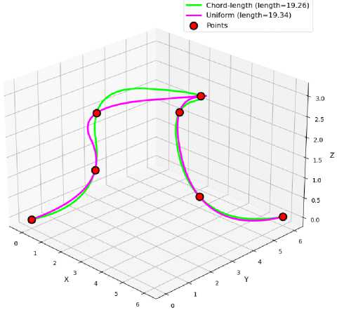
Fig.3. Comparison between uniform and chord-length knot distribution

The proposed enhanced adaptive B-Spline smoothing method addresses the shortcomings of conventional approaches through an adaptive knot placement strategy that reflects local trajectory complexity, thereby mitigating both underfitting and overfitting. In order to match the smoothed path with actual flight envelopes, physical restrictions like curvature, acceleration, and velocity are directly incorporated into the optimization goal. The strategy preserves resilience against local minima that could compromise strictly gradient-based techniques by utilizing evolutionary algorithms. A dedicated post-processing step then ensures that once a broadly optimal set of knots and control points has been found, finer-scale constraints are systematically enforced. Consequently, this method emerges as a viable solution for UAV track smoothing tasks, especially in scenarios involving noisy measurement data, high maneuverability, or dynamically changing mission demands.

In order to assess the performance and practical viability of the proposed enhanced adaptive B-Spline smoothing approach in three-dimensional (3D) environments, we developed a simulation environment in which a UAV must navigate from a designated start location S to a target location T while avoiding multiple fixed obstacles. Each obstacle fills a cubic or cylindrical volume, representing high-rise buildings, communication towers, or other structures commonly encountered in realistic 3D urban or rugged terrains. A buffer margin of five units is assigned to each obstacle to ensure that the smoothed trajectory remains safely outside any collision zone.

All trials are conducted within a simulated three-dimensional airspace measuring 2000 x 2000 x 500 meters, populated by cylindrical and cuboidal obstacles placed randomly or at predetermined coordinates. The dimensions of the simulated airspace were chosen to approximate a midsize urban environment in which a small to medium sized UAV might operate. A horizontal span of 2000 X 2000 meters represent a typical city block radius or suburban district, providing ample room for both long straight segments and nontrivial detours around obstacles. The vertical extent of 500 meters ensures that the UAV must contend with realistic changes in altitude—such as flying above low - lying buildings or under overpasses—while remaining within the operational ceiling of most commercially available multirotor platforms. These bounds strike a balance between capturing enough environmental complexity to stress - test the smoothing algorithm and keeping computation times reasonable for near - real - time evaluation.

Cylindrical and cuboidal obstacles were selected because they represent two of the most common obstacle geometries a UAV encounters in urban or rural settings. Cylindrical obstacles model structures such as communication towers, silos, or streetlight poles—objects with circular cross-sections that require careful curvature management to avoid collision. Cuboidal obstacles simulate buildings, crates, or shipping containers, all of which present right-angled faces that test a path planner’s ability to navigate around sharp edges. By including both shapes, the simulation probes the algorithm’s capacity to maintain smooth curvature in the face of convex (cylinder) and polygonal (cuboid) constraints. Randomizing obstacle placement alongside a few predetermined configurations further ensures that performance metrics are not overstated due to an overly contrived environment; instead, they reflect an algorithm that must adapt to both structured layouts (e.g., city grids) and unpredictable obstacle distributions.

The UAV’s mission is to navigate from a start point S = (0,0,20) to a target point T = (2000,1800,200) . Figure 4 illustrates a typical arrangement of obstacles in this environment.

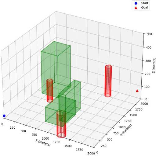
Fig.4. An illustrative layout of the environment

In evaluating the performance of path smoothing, we compare four approaches:

• •    Baseline Polyline (No Smoothing). Direct use of a path generated by a path-planning algorithm, retaining all high-angle turns and irregular steps.

• •    Uniform B-Spline. A cubic B-Spline fit with uniformly spaced knots, providing a global smoothing strategy but not accounting explicitly for curvature demands.

• •    Classical B-Spline with Fixed Knot Placement. Similar to the uniform approach but employs chord-length parameterization for knot placement, without explicit consideration of flight dynamics.

• •    Proposed Enhanced Adaptive B-Spline. Integrates adaptive knot placement with curvature-aware control point refinement to better accommodate UAV flight dynamics.

To assess smoothing quality and computational efficiency, we employ the following key metrics:

Path Length L = X^¹   ||X; ₊₁ - xll where {x/} are consecutive waypoints (or sampled spline points).

Shorter paths are generally preferable, provided they maintain acceptable smoothness.

r \     |^ ⁽U)XC ⁽U)|           . .           . . .        .        ,                                т

Maximum Curvature k(u) = 1—       !, sampled at multiple points along the trajectory. Lower Kmax dedicates more stable flight with less aerodynamic stress.

Computation Time. The time required to construct, evaluate, and iteratively refine the spline. While offline scenarios tolerate longer computation, minimizing overhead is beneficial for near-real-time or on-board replanning tasks.

Straightness Ratio, SR = p—^—^, where x _start and x _goal are the first and last waypoints. A straightness ratio of 1.0 corresponds to a perfectly straight, obstacle-free path; values greater than 1.0 indicate deviation around obstacles or detours.

Each experiment is repeated five times, varying obstacle placement or waypoints while preserving the same start/goal points. Table 2 presents the aggregated outcomes for the four methods, reporting mean values of key metrics.

Table 2. Performance of four path-smoothing methods

Method	Path Length (m)	Max Curvature ( m 1 )	Computation Time (s)	Straightness Ratio
Baseline Polyline (No Smoothing)	2984.6	0.65	0	1.107
Uniform B-Spline	2840.8	0.56	0.25	1.053
Classical B-Spline (Fixed Knots)	2803.2	0.49	0.31	1.039
Proposed Enhanced Adaptive B-Spline	2731.4	0.38	0.42	1.013

The Proposed Enhanced Adaptive B-Spline method achieves both the shortest path length and the lowest maximum curvature, underscoring its effectiveness at mitigating abrupt turns and redundant waypoint detours. It also attains the lowest straightness ratio, indicating that its trajectories most closely approximate the direct, straight-line route between start and goal. Although this approach incurs higher computation time than simpler uniform or chord-length-based fits, it substantially improves flight stability, reduces unnecessary path length, and increases straight-line efficiency. These advantages are particularly relevant for missions requiring stringent maneuverability or energy efficiency, where smoother trajectories and closer adherence to the shortest possible route directly translate into reduced aerodynamic stress and lower power consumption.

5.    Discussion

Our simulations confirmed that adaptively selecting knot vectors via a GA and then refining control points for curvature yields measurably smoother, shorter, and more feasible UAV paths than uniform or fixed‐knot strategies. These findings establish a new baseline for B‐spline smoothing under static conditions. However, several key factors must be addressed before translating these gains to real‐world UAV operations.

The path length and curvature metrics achieved by our enhanced B-spline method (Table 2) underscore its efficacy. When contextualized against advanced ML planners, our approach offers distinct advantages where verifiable properties are paramount. While ML can learn complex navigation policies [16], smoothness and strict adherence to dynamic constraints often remains a challenge without significant overhead or specialized design [19]. Conversely, our B-spline method provides direct, mathematically-grounded control over these critical trajectory characteristics, leading to more interpretable and verifiably safe paths. The GA-driven optimization, while computationally intensive, targets well-defined parameters for this explicit control. Thus, for missions prioritizing demonstrable safety, predictable dynamics, and precise trajectory refinement without extensive prior datasets for the core smoothing task, the proposed B-spline optimization presents a compelling alternative or a valuable component in hybrid planning systems.

Onboard computational limits of typical flight controllers (e.g., ARM Cortex‐M/A autopilots) and companion computers (e.g., Raspberry Pi) are far more constrained than our desktop environment. Running the GA with the same population size and generation count used in simulation could introduce unacceptable delays, particularly when rapid replanning is required. To mitigate this, one can reduce GA population size or generation count, warm-start the GA from a chord-length or uniform knot vector, or offload GA evaluation entirely to a companion computer while reserving only local curvature refinement for the flight controller. A hardware-in-the-loop (HIL) evaluation—integrating the smoothing pipeline with a standard autopilot (e.g., PX4 on a Pixhawk) and companion computer—will be essential to measure computation time, memory use, and power draw under realistic cycle‐time constraints (ideally below 250 ms for a full update in a medium‐complexity environment).

In real missions’ obstacles can move unpredictably (e.g., other UAVs, vehicles, or temporary structures). Continuously recomputing the entire B-Spline when new obstacles are detected may be too slow. A hierarchical planning framework—where a fast, reactive local planner (e.g., MPC or velocity‐obstacle method) operates at 10–20 Hz to ensure immediate collision avoidance, while the global B-Spline optimizer runs at 1–2 Hz to refine the overall trajectory—can balance safety and smoothness. Additionally, incremental GA updates that warm-start from the previous solution and adjust only a subset of knots near new obstacles can reduce computation while still adapting to environmental changes.

Real UAVs contend with sensor noise and state-estimation errors. Low-cost GPS drift, IMU bias, and vision failures in low‐lighting can lead to inaccurate waypoint data and tracking errors. To counteract this, raw waypoints should be prefiltered (e.g., sliding‐window median or Kalman filtering) before spline fitting. Moreover, incorporating uncertainty into the optimization—by treating waypoints as probabilistic regions or adding buffer margins around obstacles proportional to localization error—can reduce collision risk, though it may lengthen the planned path.

Environmental disturbances such as wind gusts and turbulence near buildings can alter the actual curvature experienced by the UAV. In simulation we enforced only kinematic constraints and fixed buffer margins; in the field, even moderate crosswinds (3–5 m/s) can induce lateral drift. Coupling the smoothing algorithm with a real-time wind estimator (e.g., an extended Kalman filter fusing IMU and airspeed data) allows dynamic adjustment of the curvature penalty and buffer margins in regions of high turbulence. If 6-DoF dynamics simulations reveal tracking errors beyond acceptable thresholds (e.g., lateral deviations > 0.5 m), then curvature constraints should be tightened or control gains retuned to maintain safe tracking under disturbances.

Finally, a structured validation protocol is necessary. We recommend:

• •    HIL Testing to quantify onboard computation and energy consumption.

• •    High-Fidelity Dynamics Simulation (6-DoF quadrotor with wind models) to measure trajectory tracking error and safety margins.

• •    Controlled Outdoor Trials (e.g., foam obstacles in open fields) to compare path quality, mission time, and power draw against baseline smoothing methods.

• •    Complex Urban Flights with static and dynamic obstacles, implementing the hierarchical planner, and measuring replanning frequency, resource use, and near-miss incidents.

6.    Conclusions

By addressing onboard compute constraints, dynamic obstacles via hierarchical planning, sensor uncertainty with filtering and buffer inflation, and environmental disturbances with wind-aware cost terms, the proposed method can be adapted for reliable, energy-efficient UAV missions. These validation steps will determine which parameter settings (GA budget, curvature limits, buffer sizes) meet real-world performance and safety requirements.

This paper introduced an Enhanced Adaptive B-Spline Smoothing Approach tailored for UAV path planning in complex three-dimensional environments. By integrating an adaptive knot placement strategy optimized via a genetic algorithm with curvature-aware control point refinement, our method effectively addresses the challenges of maintaining flight viability, ensuring smooth trajectory transitions, and minimizing aerodynamic stress. Quantitative evaluations demonstrated that, compared to uniform or fixed-knot B-Spline parameterizations, our approach yields trajectories with substantially lower maximum curvature and reduced path length, contributing to improved flight stability and efficiency. The adaptive knot placement allows for localized B-Spline refinement, accurately capturing path complexities, while integrated curvature constraints ensure dynamic feasibility.

Despite these advancements, certain limitations warrant consideration. The primary simulation studies were conducted in static environments, and while the method is designed for near-real-time re-planning, its performance with highly dynamic obstacles necessitates further investigation. The computational overhead of the genetic algorithm, though shown to be acceptable for many scenarios, could be a constraint in applications demanding extremely rapid, sub-second updates on resource-limited onboard processors. Furthermore, the current framework primarily relies on an upstream global planner for initial waypoint generation; the quality of this initial path can influence the final smoothed trajectory.

These limitations naturally point towards several promising avenues for future research. A key direction is the extension of the framework to robustly handle dynamic and unpredictable obstacles, potentially by integrating the adaptive B-Spline smoother with fast, reactive local planners or by developing incremental spline update mechanisms that efficiently respond to environmental changes. Investigating methods to reduce the computational footprint of the GA, such as exploring more efficient metaheuristics for knot optimization or leveraging parallel processing architectures more effectively, would enhance its applicability for real-time onboard execution. Further research could also focus on incorporating more sophisticated UAV dynamic models and environmental disturbances, such as wind, directly into the optimization process. Exploring hybrid approaches that combine the strengths of our mathematically-grounded B-Spline optimization with machine learning techniques for perception, high-level decision-making, or even guiding the GA's search, could lead to even more powerful and adaptive path planning solutions. Finally, extensive validation through hardware-in-the-loop simulations and real-world flight experiments in complex scenarios will be crucial to fully assess the practical performance and robustness of the proposed method.

In summary, the Enhanced Adaptive B-Spline Smoothing approach represents a significant step towards generating high-quality, dynamically feasible UAV trajectories. While acknowledging current limitations, the identified future research directions offer exciting prospects for further advancing UAV autonomy and operational safety in challenging environments.