An enhanced differential evolution algorithm with multi-mutation strategies and self-adapting control parameters

Published Online April 2019 in MECS

• I.    Introduction

  In 1995, Storn and Price presented the first differential evolution (DE) algorithm for global optimization problems [1]. It is a stochastic population-based optimization algorithm used to optimize real-parameter, real-valued functions [2]. The DE is a simple and effective algorithm that has a small number of adjustable control parameters. It has been successfully used in many engineering applications of several fields such as neural networks, signal processing, pattern recognition, image processing, bioinformatics, control systems, robotics, wireless communications, and semantic web [2-8]. Exploration and exploitation abilities of any populationbased optimization algorithm play a vital role in enhancing its accuracy and convergence speed [9]. In exploration, an optimization algorithm explores the search space of the problem globally in order to find new solutions and perform coarse refinements of the candidate solutions. In exploitation, on the other hand, it performs fine refinements in the neighborhoods of the existing solutions locally to improve the current solutions [9].

Recently, various variants of the DE algorithm have been introduced to improve its exploration and exploitation abilities. The changes of these variants are based on designing new mutation strategies and selfadapting control parameters [9-15]. However, the performance of the recent DE variants is still dependent to a great extent on the particulars of the optimization problem at hand [4, 12]. This means that one algorithm can succeed with certain problems but it may fail with other problems, implying that the algorithm lacks the required generality [4, 12]. This represents an open research point for promising attempts to devise more general optimization algorithms. A self-adapting DE algorithm (SaDE) is introduced in [3], where the selection of the strategy and the value of control parameters F and CR are not required to be pre-defined. In [10], a mutation strategy denoted by "DE/current-to-pbest" with optional external archive and adapting control parameters is proposed to form a new variant of DE called JADE. It represents a generalization of the classic "DE/current-to- best". The authors in [4] propose to employ an ensemble of mutation strategies and control parameters for the DE algorithm (EPSDE). In EPSDE, multi-mutation strategies and control parameter values with diverse characteristics are collected in a pool. An improved version of JADE, named success-history based adaptive DE algorithm (SHADE), is presented in [16]. It uses a different parameter adaptation mechanism for DE based on a history of successful control parameter settings. In [17], a competitive variant of adaptive DE, called b6e6rl, is proposed to solve the set of benchmark functions of the CEC 2013 competition. In this variant, the competitive adaptation is performed through twelve different mutation strategies and parameter settings. A modified adaptive differential evolution (ADE) is developed in [18]. It adopts the quasi-oppositional probability based on population’s variance information to tune the scaling factor (F) and the crossover rate (CR). In [19], a modified mutation strategy and a fitness induced parent selection scheme for the binomial crossover of DE with selfadapting control parameters are adopted. The proposed mutation strategy is based on the classic variant "DE/current-to-best/1" with some modifications. It is referred to as MDE_pBX. In [20], an auto-enhanced population diversity mechanism (AEPD) is proposed to be used with DE. The population diversity is enhanced by measuring the population distribution in each dimension to avoid stagnation and premature convergence issues of the DE algorithm. The authors in [11] introduce a new DE algorithm with a hybrid mutation operator and selfadapting control parameters (HSDE). The population is classified into two groups; each group has different mutation operators and self-adapting control parameters. In [21], an abstract convex underestimation-assisted multistage DE is presented. In this algorithm, the supporting vectors of some neighboring individuals are used to calculate the underestimation error. The variation of the average underestimation error is used to perform three stages of the evolutionary process with a pool of suitable candidate strategies for each stage. In [12], a DE algorithm with improved individual-based parameter setting and selection strategy is suggested. Hybrid mutation strategies with a prescribed probability and a selection strategy based on the diversity of a weighted fitness value are used. An enhanced fitness-adapting DE algorithm with a modified mutation (EFADE) is given in [22]. A triangular mutation operator is used in EFADE to achieve a good balance between exploration and exploitation.

Although there are many versions of the DE algorithm, they have many drawbacks related to their performance [4, 22]. Firstly, they are good at global exploration, but they exhibit a slow convergence at local exploitation. Secondly, they are sensitive to the choice of the mutation strategy and control parameter values; that is, they are problem dependent. Thirdly, the DE performance degrades in highdimensional optimization problems.

In the present paper, we propose a further improvement to the basic variants of DE that enhances its performance in terms of the convergence speed and accuracy, simplicity being preserved. A combination of three mutation strategies and their corresponding self-adapting control parameters is employed. The first and second mutation strategies are taken to be "DE/rand/1" and "DE/best/1". The third mutation strategy is chosen to be the average between the previous two mutation strategies. During the evolutionary process, the locations of the current, best, and worst individuals are utilized to determine a suitable mutation strategy.

This paper is organized as follows: Section II reviews the basic variants of DE. Section III presents the proposed DE algorithm. In Section IV the proposed algorithm is tested through a variety of well-known benchmark optimization functions. Finally, Section V concludes the paper.

• II.    Basic Differential Evolution Algorithm

  The procedure of the basic DE algorithm is outlined in the following four sequential phases: initialization, mutation, crossover, and selection [2325].

• A.    Initialization Phase

In this phase, a population of NP D -dimensional real-valued vectors ( NP is the population size) is randomly chosen within the search space R ^D of the optimization problem [2]. Let X ^G be the target vector that minimizes the objective function f(X) . It can be represented as[25]:

where x ^G is the j^th ( j=1, 2,. . . , D ) component of the i^th ( i = 1, 2, . . . ,NP ) population vector at the current generation G ( G = 0, 1, . . . ,G max ). G max is the maximum number of generations. The initial population at generation G =0 can be generated as:

j,i       j,min             j,i     ,           j,max       j,min where x and x are the minimum and maximum bounds of the jth component in the search space, respectively, and rand , e[0,1] is a uniformly distributed random number within the range [0,1].

• B.    Mutation Phase

In the mutation phase, the mutant (or donor) vector V G ^{+ 1} is created for each target vector X f . The most common mutation strategies are generated using the following equations [26, 27]:

"DE/best/1"

• V G ^{+ 1} = X GL, + F * ( x G - X G2 )          (3)

"DE/rand/1"

ViG+1 = XG + F x( XG - XG)

"DE/best/2"

ViG+1 = XL + Fx(XG -XG)+Fx(XG -XG)

"DE/rand /2"

G+1   VG      VG  VG       VGV

VI   = Xr 1 + F X( Xr 2 - Xr 3 ) + F X( Xr 4 - Xr 5 )

"DE/current-to-best /1"

VG+1 = XG + Fx(X^ -XG)+Fx(XG -XG)

where F e [0, 2] is a control parameter called the mutation scaling factor. r1, r2, r3, r4 and r5 are random integers within the range [1, NP ], such that r1 ≠ r2 ≠ r3 ≠ r4 ≠ r5 ≠ i. X ^G is the best individual that has a minimum objective function value at the current generation G .

• C.    Crossover Phase

In this phase, the trial vector U G ^{+ 1} is generated by exchanging the elements of the target vector X ^G with the elements of the mutant vector V G ^{+ 1} as [24, 28]:

• V G ^{+ 1}, if rand j [ 0,1 ] < CR or j = j^ ₍₈₎ X ^G , otherwise

  
  
  

where CR e [0, 1] is a control parameter called the crossover rate and j_md e [0, D ] is a random integer used to ensure that the trial vector U G ^{+ 1} and the target vector X ^G are different.

i

• D.    Selection Phase

In this phase, the target vector X ^G is compared with the trial vector U G ^{+ 1}, and the fittest one that has a lower objective function value will be chosen to represent the target vector X G ^{+ 1} in the next generation. The selection phase is performed using Equation (9) [2]:

X G ^{+ 1} = <

U G ^{+ 1}, if f ( U G ^{+ 1} ) < f ( X G )

X ^G ,             otherwise

where f is the objective function to be optimized.

• III.    Proposed Approach

The performance of a DE algorithm depends on two issues. The first issue is concerned with the choice of a suitable mutation strategy for the optimization problems that have distinct properties. The second issue is concerned with the adaptation of the control parameters that affect the behavior of the mutation strategy and the crossover phase [4]. Therefore, the basic DE algorithm with a single mutation strategy and fixed control parameters can be modified to be more flexible and efficient [12]. This enhancement can be achieved using multi-mutation strategies and self-adapting control parameters to make a balance between the exploration and exploitation abilities.

Motivated by these facts, we propose an enhanced DE algorithm, denoted by MSaDE, with multi-mutation strategies and self-adapting control parameters. The proposed algorithm makes use of three mutation strategies with their associated self-adapting control parameters. The first one increases the exploration ability which is related to the global search. The second mutation strategy increases the exploitation ability which is related to the local search. The third one achieves a balance between the exploration and exploitation abilities. Selection between these three strategies is done automatically with the help of the current, best, and worst individuals at the current generation.

• A.    Proposed Multi-mutation Strategies

The location of the current individual in the search space is a good guide metric to determine if this individual is to be assigned to the mutation strategy at high rates of exploration or exploitation.

Two absolute differences are calculated: (1) the absolute difference between the objective function of the current and worst individuals CW G = f ( X G ) - f ( X Gorn )| , (2) the absolute difference between the objective function of current and best individuals CB G = f ( X G ) - f ( X G_st )| . According to the result, the current individual will be assigned to one of three mutation strategies: "DE/rand/1", "DE/best/1", or the average mutation. Five randomly chosen individuals ( X^G , X^G , X^G , X^G , and X ^G ) in addition to the best individual ( X ^G ) are used to form the proposed mutation strategies. X ^G and X ^G are used as the base vectors of the first two mutations "DE/rand/1" and "DE/best/1", respectively. The other individuals are used to create two difference vectors: ( X G - X G ) and ( X G - X G ) . The difference vector with a higher objective function value is assigned to the first mutation "DE/rand/1" to improve the exploration search ability. It increases the ability for searching new regions over a large search volume. The difference vector with a lower objective function value is assigned to the second mutation "DE/best/1" to improve the exploitation search ability. It increases the ability for searching new solutions in a small or immediate neighborhood. The average of the two difference vectors is assigned to the third mutation to balance the exploration and exploitation abilities. The proposed three mutation strategies to generate the mutant vector V G ^{+ 1} ( i = 1, 2, . . ., NP ) are defined as:

X GG + F G X HDF , if CB^G >  CW G and rand, [ 0,1 ] < T

V G + i

X ^ , + F G X LDFf , if CB^G <  CW G and rand [ 0,1 ] >  T mean ( X G , X G ) + F G x mean ( HDF^G , LDF^G ) , otherwise (10)

where HDF^G and LDF^G are the two difference vectors with higher and lower objective function values, respectively.

_G [ X G - x G , iff(x G - x G >> f(x G - x^A

G         r 2       r 3             r 2       r 3            r 4       r 5       (11)

[ X G - X G ,                       otherwise

GG  GG  GG

LDF G = <  ^r 4 ^r5 , ^{J J} V ^{r 2 r}3' ^J v ^{r 4      r}5'    (12)

[ X G - X G ,                       otherwise

F^G , F^G , and F ^G are the scaling factors of the proposed mutation strategies. Each scaling factor is randomly chosen for every mutant vector from a predefined range of values. These ranges suit the exploration and exploitation abilities of the selected mutation strategy. T is a predefined threshold, and mean () is the arithmetic mean. The mutant vector is generated using only one mutation of the three mutation strategies depending on the values of the absolute differences CB ^G and CW ^G with a probability threshold condition T .

• B.    Parameter Adaptation Strategy

The control parameter values of the scaling factor F and the crossover rate CR affect the performance of the DE algorithm. For the same optimization problem, different rates of exploration and exploitation are required during the optimization process [9]. Therefore, it is recommended to tune the values of the control parameters at every generation to guide the search direction.

The proposed mutation strategies have three directions of search: (1) search with a high exploration rate that is achieved through the first mutation strategy, (2) search with a high exploitation rate that is achieved through the second mutation strategy, (3) search with a balanced rate between them that is achieved through the third mutation strategy. For each target vector X ^G at the current generation G , one of the three mutation strategies is selected with suitable values of the scaling factor and crossover rate.

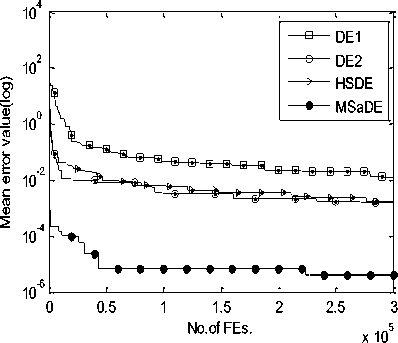
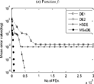
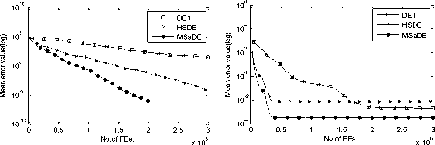
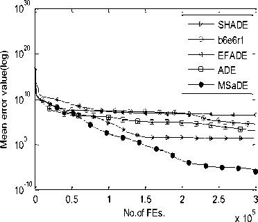
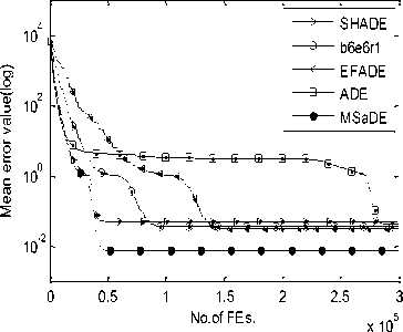
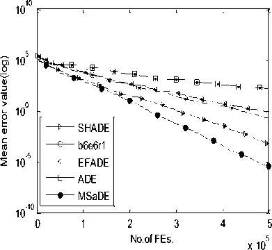
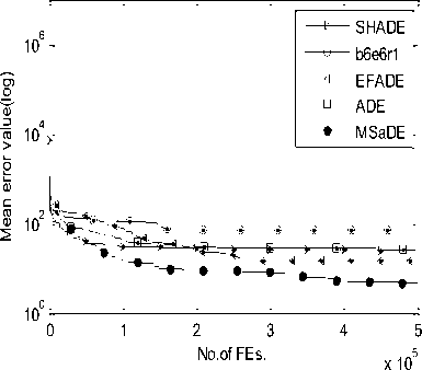
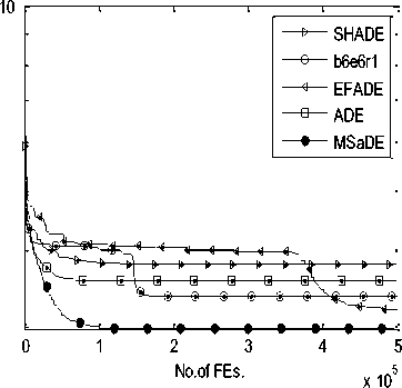
So, we choose the values of these control parameters randomly from three predefined ranges. Several trials over a large number of benchmark functions with different characteristics are made to determine these ranges. The first range of the control parameters is taken as F1 = [0.7 0.8 0.9 0.95 1.0] and CR1 = [0.05 0.1 0.2 0.3 0.4] which is suitable when choosing the first mutation strategy (i.e. FG e F1 and CRG e CR1). The second range is taken as F2 = [0.1 0.2 0.3 0.4 0.5] and CR2 = [0.8 0.85 0.9 0.95 1.0] which is suitable when choosing the second mutation strategy (i.e. FG e F2 and CR^ e CR2). The third range is taken as F3 = [0.3 0.4 0.5 0.6 0.7] and CR3 = [0.4 0.5 0.6 0.7 0.8] which is suitable when choosing the third mutation strategy (i.e. FG e F3 and CRG e CR3). During the evolution process, the values of the control parameters that will be used in the next generation are updated or remain unchanged according to the result of the selection phase. If the trial vector is fitter than the target vector (i.e. f (UG +1 )

• IV.    Experimental Study and Discussion

  Our algorithm MSaDE is applied to minimize three sets of well-known benchmark functions with different characteristics. The first set of benchmark functions consists of 13 traditional functions, named J1, f₂, „., f₁₃. These functions are the first thirteen functions chosen from [11], and they are called Sphere, Schwefel 2.22, Schwefel 1.2, Schwefel 2.21, Rosenbrock, Step, Quartic with noise, Schwefel 2.26, Rastrigin, Ackley, Griewank, Generalized Penalized Function 1, and Generalized Penalized Function 2, respectively. The optimal value of the function f₈ is -12569.5, and the remaining functions have optimal values equal to zero. Functions f₈ - f₁₃ are multimodal, the Rosenbrock function (f₅) is unimodal for D = 2 and 3 but multimodal in higher dimensions [29]. The other functions are unimodal.

The second set of benchmark functions consists of 10 special functions, named f_c1, f_c2 „., f_c10. These functions are the first ten functions from CEC2005 [30, 31].

Functions fc1 - fc5 are unimodal and functions fc6 - fc10 are multimodal. The third set of benchmark functions consists of 15 special functions chosen from CEC2013 [31, 32], named fC^, fcc2, ^, f^o, fcc21, U2, ^, fcc25. The subscript number of the function name refers to its order according to the CEC2013 benchmark functions. Functions fcc1 - fcc5 are unimodal, functions fcc6 - fcc10 are multimodal, and functions fcc21 - fcc25 are compositions.

MSaDE is compared with the standard "DE/rand/1/bin" and some efficient state-of-the-art DE algorithms with a hybrid mutation operator and self-adapting control parameters (HSDE) [11] over the first and second set of benchmark functions with dimension D = 30. The third set of benchmark functions with dimension D = 30 and 50 is used to compare MSaDE with four state-of-the-art DE algorithms: a competitive variant of adaptive DE (b6e6rl) [17], an enhanced fitness-adapting DE algorithm with a modified mutation (EFADE) [22], Success-History based Adaptive DE algorithm (SHADE) [16], and a modified adaptive differential evolution (ADE) [18].

All comparisons are made in terms of the mean and standard deviation (STD) of the error. The error in a run is calculated as f (xbest) -    f (x ), where xbest is the best solution in a run and x* is the global minimum of the function. We use the same results of the mean and standard deviation (STD) of the error for the other DE algorithms as in their papers. Furthermore, the convergence rate for some selected functions is illustrated.

To achieve a fair comparison between MSaDE and the other DE algorithms, we use two nonparametric statistical tests in the comparisons: Wilcoxon signed-rank and Friedman tests [33]. Wilcoxon signed-rank test computes R⁺, R^-, and p-value, where R⁺ is the sum of ranks that

MSaDE performs better than the other algorithm, R^- is the sum of ranks that MSaDE performs worse than the other algorithm, and p-value refers to the significant difference between each pair of algorithms (MSaDE and one of the other algorithms) with a significance level α. The considerable difference exists only if p-value < α. Friedman test is used to rank all algorithms from best to worst over all the tested functions. The algorithm that has a minimum rank value is the best and the one that has a maximum rank value is the worst.

Algorithm 1. Pseudo-code of the proposed MSaDE algorithm

%Gmax: Maximum number of generation

%MS_t: Indicator for the selected mutation

• 1:    Generate the initial population P° = [А^л®_ЭХ °, ... , АГ®_р ]

• 2:    Set the generation number G = 0

• 3:    Set the threshold 7=0.4

• 4:    Set the ranges of vectors Fi, Fi, Fj, CRi. CRi, and CR3 as we proposed in section III

• 5:    Select randomly the initial values of the control parameters Ff\ , F^G_t , F^ ,CR^G_t ,CR‘ and CR^G₃ from F1, F», F3, CR,, CR2, and CRj₂ respectively.

• 6:    Evaluate : f (%f ) , r=l, 2,..., NP

• 7:    r~ w hile G < Gmax do

  8:

  9:

  
  

  Mutation setup

  
  

  10:

  
  

  12:

  
  

  for i=l toTVPdo

  Choose randomly five individuals X^G_t , X^G₂, X^G₃, X^, and X ^G_s Determine the best individual (XL ) and die worst individual (X^G„u Calculate CB° = jf ^X° ^-f ^Х^ )| and CW = = |f (Xf )-/

  Calculate HDF⁽' and LDF^G using Eqs. 11 and 12, respectively

  
  

  13:

  
  

  Г/

  
  

^° + Л" ^HDF" and Set ->MS, = 1, if CB“ ^CW° and rand, [0.1]XL *F?>xLDFf and Set ^MS, = 2,ifCB” [0.1] >7, mean(X ° ,XL l + ^A *meanG ,LDF,^G )and Set —> MS, = 1,otherwise,

14:

end for

15:

16:

17:

18:

19:

20:

21:

Crossover setup

: for i=l to NP do

Generate j„„a= randiiD, 7)

for у = 1 to D do

{PT⁷/¹, if rand ГОЛИСЯ* or J = /' , f *         У L                         a J rota

XG^, otherwise end for end for

Selection setup for i=l to NP do

UL' and Set ^ F^G*' =F“ .CR“Ls =CR°_ms , if f kuL'A^f (X ^G )

22:

23:

24:

25:

XG aid Set —» F‘‘L = FMS {/_,        = CR„, [d. ], otherwise, t                        I                  I rand                          Мл, l rand M                  ~

% where 1^^ and J_rontl are random integers € [1 ,5]

end for

Next generation (G=G-*-l^ end while

• A.    Test Setup

  The simulation results are obtained using a digital computer with CPU core i3 (2.4 GHz, 3M cache) and 4 GB of RAM in MATLAB R2007b Runtime Environment. The maximum number of evaluations of the objective function (FEs) = 10,000×D for all sets of benchmark functions. The population size (NP) of MSaDE in the first, second, and third sets of benchmark functions is NP = 50, 100, and 100, respectively. The threshold T is set as 0.4 for MSaDE algorithm in each set of the benchmark

functions.

The average of the results is obtained over 30 independent runs for the first set of benchmark functions, 25 independent runs for the second set, and  51

independent runs for the third set. For the third set, we set all values of the error that is less than 10-8 to zero as in CEC2013. In order to achieve a fair comparison as in [34], we use two different settings of the control parameters NP, F, and CR for the "DE/rand/1/bin" algorithm that is used in the first set of benchmark functions. In the first setting, the control parameters are fixed to NP=30, CR=0.9, and F=0.9 for all functions in this set, and we refer to the "DE/rand/1/bin" algorithm as DE1. In the second setting, NP is fixed to 25 while F and CR are tuned from one function to another to suit the different properties of functions.

We refer to the "DE/rand/1/bin" algorithm of the second setting as DE2, and we use the best values for F and CR that are reached in [34]. In the second set of benchmark functions, the control parameter settings of DE are fixed to NP=30, CR=0.9, and F=0.9 as in CEC2005, and also we refer to it as DE1. The settings for the other

DE algorithms are the same as in their papers. We use the arithmetic signs "+", "=", and "-" in the results to show that MSaDE performs better than, similar to, or worse than the other variant of DE, respectively. Wilcoxon signed-rank test is applied at a significance level of α=0.05 and α=0.1.

• B.    Results of First Set of Benchmark Functions

For the 13 benchmark functions of the first set, the results of the mean and STD of the error for MSaDE, DE1, DE2 and HSDE are listed in Table 1.

Table 1. Mean and STD of error for the first set of benchmark functions with D=30

f(x)		DE1		DE2				HSDE		MSaDE
		Mean (STD)		F	CR	Mean (STD)		Mean (STD)		Mean (STD)
Unimodal Functions	f1	6.57E -15 (1.13E -14)	+	0.5	0.3	0.00E+00 (0.00E+00)	=	6.08E -52 (8.33E -52)	+	0.00E+00 (0.00E+00)
	f2	5.13E -09 (5.33E -09)	+	0.5	0.3	1.74E-108 (2.23E-108)	+	5.82E -38 (6.18E -38)	+	0.00E+00 (0.00E+00)
	f3	2.39E -01 (2.77E -01)	+	0.9	0.9	1.20E -03 (1.40E -03)	+	7.41E -33 (2.52E -32)	+	0.00E+00 (0.00E+00)
	f4	1.88E+00 (4.54E -01)	+	0.6	0.6	6.66E -14 (3.53E -14)	+	5.01E -19 (1.11E -18)	+	0.00E+00 (0.00E+00)
	f5	2.97E+01 (2.82E+01)	+	0.6	0.8	4.66E+00 (3.06E+00)	+	0.00E+00 (0.00E+00)	-	5.40E -29 (0.00E+00)
	f6	5.14E -15 (7.20E -15)	+	0.5	0.3	0.00E+00 (0.00E+00)	=	0.00E+00 (0.00E+00)	=	0.00E+00 (0.00E+00)
	f7	1.75E -02 (5.80E -03)	+	0.3	0.3	1.80E -03 (1.10E -03)	+	2.27E -03 (1.06E -03)	+	3.00E -05 (2.83E -05)
Multimodal Functions	f8	2.77E+02 (1.62E+02)	+	0.9	0.3	0.00E+00 (0.00E+00)	=	0.00E+00 (0.00E+00)	=	0.00E+00 (0.00E+00)
	f9	2.39E+01 (6.97E+00)	+	0.9	0.1	0.00E+00 (0.00E+00)	=	0.00E+00 (0.00E+00)	=	0.00E+00 (0.00E+00)
	f10	1.06E -08 (8.00E -09)	+	0.5	0.3	2.67E -15 (0.00E+00)	+	1.44E -14 (3.78E -15)	+	1.42E -15 (0.00E+00)
	f11	3.90E -03 (6.10E -03)	+	0.5	0.3	0.00E+00 (0.00E+00)	=	7.22E -03 (8.30E -03)	+	0.00E+00 (0.00E+00)
	f12	4.10E -03 (2.05E -02)	+	0.5	0.3	0.00E+00 (0.00E+00)	=	1.57E -32 (1.11E -47)	+	0.00E+00 (0.00E+00)
	f13	5.54E+01 (2.41E+01)	+	0.5	0.3	0.00E+00 (0.00E+00)	=	7.39E -53 (3.10E -52)	+	0.00E+00 (0.00E+00)
	+/-/=	13/0/0		6/0/7				9/1/3

Table 2. Average ranks of MSaDE and other algorithms using

Friedman's test for the first set of benchmark functions with D = 30

f(x)	Rank	Algorithm	Average Rank
Unimodal Functions	1	MSaDE	1.36
	2	DE2	2.36
	3	HSDE	2.43
	4	DE1	3.86
Multimodal Functions	1	MSaDE	1.58
	2	DE2	1.75
	3	HSDE	2.83
	4	DE1	3.83
All Functions	1	MSaDE	1.46
	2	DE2	2.08
	3	HSDE	2.62
	4	DE1	3.85

Compared to DE1, the accuracy of MSaDE is the best for all tested functions in this set. Compared to DE2, the accuracy of MSaDE is the best for the six functions f2-f5, f7, and f10 of the set and the same for the seven functions f1, f6, f8, f9, and f11-f13. Compared to HSDE, the accuracy of MSaDE is the best for the nine functions f1-f4, f7, and f10-f13 of the set and the same for the three functions f6, f8, and f9. The accuracy of HSDE for the function f5 is better than MSaDE. The average ranks using Friedman's test for MSaDE, DE1, DE2 and HSDE are listed in Table 2. This test is applied to three cases: (1) only the unimodal functions are considered, (2) only the multimodal functions are considered, (3) all of the functions are considered. According to the results of Friedman's test for all the three cases, the other algorithms are ordered from best to worst: MSaDE is the first, DE2 is the second, HSDE is the third, and DE1 is the last.

The results of Wilcoxon’s test are listed in Table 3. Comparing MSaDE to all other DE algorithms as two pairs, the results show that its values of R+ > R- for all the pairs at the significance levels α=0.05 and α=0.1. This means that MSaDE accuracy is significantly better than the accuracy of the other DE algorithms. The convergence curves for functions f7 and f11 are shown in Fig.1. The mean of error over 30 runs is plotted in a log scale on the vertical axis for each number of function evaluations FEs of the horizontal axis.

Table 3. Results of Wilcoxon’s test for the first set of benchmark functions with D = 30

Algorithm	+/-/=	R+	R-	p value	α=0.05	α=0.1
MSaDE versus DE1	13/0/0	91	0	0.000	Yes	Yes
MSaDE Versus DE2	6/0/7	21	0	0.028	Yes	Yes
MSaDE versus HSDE	9/1/3	50	5	0.022	Yes	Yes

As shown in Fig.1, MSaDE reaches very fast the optimal solution with large differences than the other DE algorithms.

(b) Function f11

Fig.1. Convergence curves for functions f7 and f11

• C.    Results of Second Set of Benchmark Functions

The results of the mean and STD of the error for MSaDE, DE1, and HSDE, over the 10 benchmark functions of the second set, are listed in Table 4. HSDE has the same accuracy as MSaDE for fc1 and has the best accuracy for fc2, and fc9. For the remaining functions, the accuracy of MSaDE is the best among DE1 and HSDE. The average ranks for MSaDE, DE1, and HSDE using Friedman's test are listed in Table 5. Three cases are considered in this test: (1) only the unimodal functions are considered, (2) only the multimodal functions are considered, (3) all of the functions are considered. According to the results of Friedman's test for all the three cases, the other algorithms are ordered from best to worst: MSaDE is the first, HSDE is the second, and DE1 is the last. The results of Wilcoxon’s test are listed in Table 6. Comparing MSaDE to DE1 and HSDE as two pairs, the results show that its values of R⁺ > R^- for all of the two pairs.

According to Wilcoxon’s test, the pair algorithms MSaDE versus HSDE have a considerable difference at levels α=0.05 and α=0.1. For the pair MSaDE versus DE1, the considerable difference exists only at the significance level α=0.1. This means that MSaDE is considerably more accurate than the other algorithms. The convergence curves for functions fc4 and fc7 are shown in Fig.2. The mean of error over 25 runs is plotted in a log scale on the vertical axis for each number of function evaluations FEs of the horizontal axis. As shown in Fig.2, MSaDE has the fastest convergence rate with a high accuracy compared to the other algorithms.

Table 4. Mean and STD of error for the second set of benchmark functions (CEC2005) with D=30

f(x)		DE1		HSDE		MSaDE
		Mean (STD)		Mean (STD)		Mean (STD)
Unimodal Functions	fc1	5.11E -14 (1.72E -14)	+	0.00E+00 (0.00E+00)	=	0.00E+00 (0.00E+00)
	fc2	2.54E -01 (2.70E -01)	+	2.29E -22 (5.32E -22)	-	1.13E -13 (4.97E -14)
	fc3	9.65E+05 (5.11E+05)	+	5.37E+04 (2.33E+04)	+	1.36E+04 (8.87E+03)
	fc4	3.18E+01 (3.21E+01)	+	1.50E -04 (7.11E -04)	+	4.34E -12 (4.29E -12)
	fc5	2.49E+02 (1.77E+02)	+	5.33E+02 (3.90E+02)	+	1.87E -05 (2.37E -05)
Multimodal Functions	fc6	2.82E+01 (2.63E+01)	+	1.59E -01 (7.97E -01)	+	3.06E -13 (5.77E -13)
	fc7	3.60E -03 (6.10E -03)	+	1.00E -02 (1.13E -02)	+	7.39E -04 (2.30E -03)
	fc8	2.09E+01 (6.54E -02)	+	2.09E+01 (3.37E -02)	+	2.08E+01 (5.65E -02)
	fc9	2.11E+01 (6.96E+00)	-	0.00E+00 (0.00E+00)	-	2.30E+01 (1.50E+01)
	fc10	1.92E+02 (5.88E+01)	+	4.70E+01 (1.16E+01)	+	4.26E+01 (1.06E+01)
	+/-/=	9/1/0		7/2/1

Table 5. Average ranks of MSaDE and other algorithms using Friedman's test for the second set of benchmark functions (CEC2005) with D = 30

f(x)	Rank	Algorithm	Average Rank
Unimodal Functions	1	MSaDE	1.30
	2	HSDE	1.90
	3	DE1	2.80
Multimodal Functions	1	MSaDE	1.40
	2	HSDE	2.00
	3	DE1	2.60
All Functions	1	MSaDE	1.35
	2	HSDE	1.95
	3	DE1	2.70

Table 6. Results of Wilcoxon’s test for the second set of benchmark functions (CEC2005) with D = 30

Algorithm	+/-/=	R+	R-	p value	α=0.05	α=0.1
MSaDE versus DE1	9/1/0	50	5	0.06	No	Yes
MSaDE versus HSDE	7/2/1	38	7	0.02	Yes	Yes

D. Results of Third Set of Benchmark Functions

(a) Function fc4

(b) Function fc7

Fig.2. Convergence curves for functions fc4 and fc7

The third set of benchmark functions contains 15 special functions with dimensions D = 30 and 50, chosen from CEC2013. The results of this set for D = 30 are explained as follows. The mean and STD of the error for MSaDE, b6e6rl, EFADE, SHADE, and ADE are listed in Table 7. Among all DE algorithms, the performance of MSaDE in terms of accuracy is the best for the functions fcc2 - fcc4, fcc6, fcc7, fcc10, fcc21 and fcc23. MSaDE and ADE have the same best value of the mean error over the function fcc24.

The performance over the two functions fcc1 and fcc5 is nearly the same for all other algorithms. For the remaining functions of the set, MSaDE performance is slightly less than the other algorithms. The results of Wilcoxon’s test are listed in Table 8. Comparing MSaDE to all other DE algorithms pairwise, the results show that its values of R+ > R- for all of the four pairs with a significance level α=0.05 and α=0.1. These results ensure that MSaDE is considerably more accurate than the other DE algorithms. The convergence curves for functions fcc3, fcc10, and fcc23 are shown in Fig.3.

The mean of error over 51 runs is plotted in a log scale on the vertical axis for each number of function evaluations FEs of the horizontal axis. Fig.3 shows that MSaDE converges very fast to the optimal solution when compared to the other DE algorithms.

The results of this third set for D = 50 are explained as follows. The mean and STD of the error for MSaDE, b6e6rl, EFADE, SHADE, and ADE are listed in Table 9. Among all DE algorithms, the accuracy of MSaDE is the best for functions fcc2-fcc4, fcc7, fcc9, fcc10, and fcc23-fcc25. The best value of the mean error for functions f_cc6, f_cc8, and f_cc22 is achieved by SHADE with a slighter difference than MSaDE. EFADE has the best accuracy over the function fcc21. The performance over the two functions fcc1 and fcc5 is nearly the same for all other algorithms. The results of Wilcoxon’s test are listed in Table 10. Comparing MSaDE to b6e6rl, EFADE, SHADE, and ADE pairwise, the results show that its values of R⁺ > R^- for all of the four pairs. For the pair MSaDE versus SHADE, a considerable difference exists only at the significance level α=0.1. The other remaining pairs have a considerable difference at levels α=0.05 and α=0.1. These results show that MSaDE is considerably more accurate than the other DE algorithms. The convergence curves for functions fcc4, fcc7, and fcc25 are shown in Fig.4. The mean of error over 51 runs is plotted in a log scale on the vertical axis for each number of function evaluations (FEs) of the horizontal axis. Fig.4 shows that MSaDE achieves a high convergence rate with more accuracy over the other DE algorithms. Friedman's test is applied to the functions of the third set through three cases of these functions. The first case uses the functions of the set with D=30, the second case uses the functions with D=50, and the last case uses the functions with D=30 and D=50. According to these three cases, the average ranks for MSaDE, b6e6rl, EFADE, SHADE, and ADE using Friedman's test are listed in Tables 11, 12, and 13, respectively. The results for each case of the test are obtained considering four classifications of the tested functions: unimodal, multimodal, composition, and all functions. For all cases and classifications of the third set of functions, MSaDE has the first rank among all other DE algorithms.

Table 8. Results of Wilcoxon’s test for the third set of benchmark functions (CEC2013) with D = 30

Algorithm	+/-/=	R+	R-	p value	α=0.05	α=0.1
MSaDE versus b6e6rl	11/1/3	69	9	0.019	Yes	Yes
MSaDE versus EFADE	12/1/2	80	11	0.016	Yes	Yes
MSaDE versus SHADE	11/2/2	76	15	0.033	Yes	Yes
MSaDE Versus ADE	10/2/3	68	10	0.023	Yes	Yes

Table 7. Mean and STD of error for the third set of benchmark functions (CEC2013) with D=30

f(x)		b6e6rl		EFADE		SHADE		ADE		MSaDE
		Mean (STD)		Mean (STD)		Mean (STD)		Mean (STD)		Mean (STD)
Unimodal functions	fcc1	0.00E+00 (0.00E+00)	=	0.00E+00 (0.00E+00)	=	0.00E+00 (0.00E+00)	=	0.00E+00 (0.00E+00)	=	0.00E+00 (0.00E+00)
	fcc2	6.99E+04 (4.41E+04)	+	2.67E+04 (1.53E+04)	+	9.00E+03 (7.47E+03)	+	2.11E+06 (1.55E+06)	+	7.60E+03 (9.31E+03)
	fcc3	4.36E+03 (1.35E+03)	+	9.10E+05 (2.41E+06)	+	4.02E+01 (2.13E+02)	+	1.64E+03 (2.83E+03)	+	4.09E -05 (1.26E -04)
	fcc4	1.80E -02 (2.88E -02)	+	3.37E+00 (3.78E+00)	+	1.92E -04 (3.01E -04)	+	1.69E+04 (2.84E+03)	+	2.74E -07 (5.44E -07)
	fcc5	0.00E+00 (0.00E+00)	=	0.00E+00 (0.00E+00)	=	0.00E+00 (0.00E+00)	=	1.39E -07 (1.86E -07)	+	0.00E+00 (0.00E+00)
Multimodal functions	fcc6	5.24E+00 (9.90E+00)	+	6.59E+00 (4.19E+00)	+	5.96E -01 (3.73E+00)	+	8.29E+00 (5.81E+00)	+	2.65E -04 (8.35E -04)
	fcc7	2.44E+01 (8.96E+00)	+	5.07E+00 (3.62E+00)	+	4.60E+00 (5.39E+00)	+	1.29E+00 (1.21E+00)	+	5.61E -01 (7.57E -01)
	fcc8	2.09E+01 (4.72E -02)	=	2.10E+01 (4.65E -02)	+	2.07E+01 (1.76E -01)	-	2.09E+01 (4.81E -02)	=	2.09E+01 (3.58E -02)
	fcc9	2.86E+01 (1.15E+00)	+	1.51E+01 (3.63E+00)	+	2.75E+01 (1.77E+00)	+	6.29E+00 (3.27E+00)	-	1.15E+01 (1.34E+01)
	fcc10	1.91E -02 (1.33E -02)	+	3.48E -02 (2.04E -02)	+	7.69E -02 (3.58E -02)	+	2.16E -02 (1.35E -02)	+	7.90E -03 (9.30E -03)
Composition functions	fcc21	2.96E+02 (8.55E+01)	+	3.38E+02 (8.93E+01)	+	3.09E+02 (5.65E+01)	+	3.19E+02 (6.26E+01)	+	2.70E+02 (4.83E+01)
	fcc22	1.23E+02 (1.63E+01)	-	2.56E+02 (1.46E+02)	-	9.81E+01 (2.52E+01)	-	2.49E+03 (3.86E+02)	+	1.03E+03 (3.27E+02)
	fcc23	5.00E+03 (4.06E+02)	+	3.84E+03 (1.08E+03)	+	3.51E+03 (4.11E+02)	+	5.80E+03 (5.04E+02)	+	3.38E+03 (4.07E+02)
	fcc24	2.51E+02 (1.38E+01)	+	2.13E+02 (7.74E+00)	+	2.05E+02 (5.29E+00)	+	2.02E+02 (1.39E+00)	=	2.02E+02 (5.48E+00)
	fcc25	2.75E+02 (1.76E+01)	+	2.61E+02 (6.95E+00)	+	2.59E+02 (1.96E+01)	+	2.29E+02 (2.07E+01)	-	2.44E+02 (3.74E+00)
	+/-/=	11/1/3		12/1/2		11/2/2		10/2/3

(a) Function fcc3

(b) Function fcc10

SHADE b6e6r1 EFADE ADE MSaDE

103 I-----------------:----------------г----------------г-----------------г----------------г1

0.5       1       1.5       2       2.53

• (c) Function fcc23

  Fig.3. Convergence curves for functions fcc3, fcc10 and fcc23 (D=30)

  
  

  Table 9. Mean and STD of error for the third set of benchmark functions (CEC2013) with D=50

f(x)		b6e6rl		EFADE		SHADE		ADE		MSaDE
		Mean (STD)		Mean (STD)		Mean (STD)		Mean (STD)		Mean (STD)
Unimodal functions	fcc1	0.00E+00 (0.00E+00)	=	0.00E+00 (0.00E+00)	=	0.00E+00 (0.00E+00)	=	0.00E+00 (0.00E+00)	=	0.00E+00 (0.00E+00)
	fcc2	3.23E+05 (1.56E+05)	+	1.72E+05 (5.48E+04)	+	2.65E+04 (1.13E+04)	+	2.04E+05 (7.67E+04)	+	1.95E+04 (7.96E+04)
	fcc3	8.61E+06 (2.33E+07)	+	5.70E+06 (6.70E+06)	+	8.79E+05 (1.96E+06)	+	7.47E+06 (7.59E+06)	+	5.15E+05 (6.68E+05)
	fcc4	2.32E-01 (3.12E-01)	+	6.16E+00 (5.24E+00)	+	1.61E -03 (1.41E -03)	+	2.20E+02 (9.58E+01)	+	4.59E -04 (3.63E -04)
	fcc5	0.00E+00 (0.00E+00)	=	0.00E+00 (0.00E+00)	=	0.00E+00 (0.00E+00)	=	1.39E -03 (1.86E -03)	+	0.00E+00 (0.00E+00)
Multimodal functions	fcc6	4.34E+01 (1.43E-14)	=	4.34E+01 (7.83E-10)	=	4.28E+01 (5.52E+00)	-	7.35E+01 (2.80E+01)	+	4.34E+01 (4.75E -13)
	fcc7	8.26E+01 (1.55E+01)	+	1.80E+01 (7.26E+00)	+	2.33E+01 (9.32E+00)	+	2.07E+01 (9.15E+00)	+	1.33E+01 (8.52E+00)
	fcc8	2.11E+01 (4.65E-02)	=	2.11E+01 (3.68E-02)	=	2.09E+01 (1.68E -01)	-	2.11E+01 (3.53E -02)	=	2.11E+01 (4.52E -02)
	fcc9	5.67E+01 (2.57E+00)	+	3.28E+01 (4.67E+00)	+	5.54E+01 (1.98E+00)	+	2.60E+01 (3.04E+00)	+	1.58E+01 (1.88E+00)
	fcc10	3.54E-02 (1.85E-02)	+	6.98E-02 (3.74E-02)	+	7.36E-02 (3.67E-02)	+	5.98E -01 (3.42E -01)	+	3.23E -02 (2.25E -02)
Composition functions	fcc21	4.60E+02 (4.10E+02)	-	3.53E+02 (3.19E+02)	-	8.45E+02 (3.63E+02)	+	9.65E+02 (1.43E+02)	+	6.19E+02 (4.82E+02)
	fcc22	3.60E+01 (2.44E+01)	+	8.84E+02 (5.22E+02)	+	1.33E+01 (7.12E+00)	-	7.72E+03 (8.46E+02)	+	2.37E+01 (5.80E+02)
	fcc23	9.77E+03 (5.33E+02)	+	7.35E+03 (1.53E+03)	+	7.63E+03 (6.58E+02)	+	1.17E+04 (1.47E+03)	+	6.60E+03 (7.29E+02)
	fcc24	3.33E+02 (1.54E+01)	+	2.45E+02 (1.10E+01)	+	2.34E+02 (1.01E+01)	+	2.78E+02 (1.82E+01)	+	2.33E+02 (1.16E+01)
	fcc25	3.64E+02 (2.08E+01)	+	3.27E+02 (1.15E+01)	+	3.40E+02 (3.08E+01)	+	3.53E+02 (1.71E+01)	+	2.91E+02 (4.43E+00)
	+/-/=	10/1/4		10/1/4		10/3/2		13/0/2

Table 10. Results of Wilcoxon’s test for the third set of benchmark functions (CEC2013) with D = 50

Algorithm	+/-/=	R+	R-	p value	α=0.05	α=0.1
MSaDE versus b6e6rl	10/1/4	58	8	0.012	Yes	Yes
MSaDE Versus EFADE	10/1/4	59	7	0.012	Yes	Yes
MSaDE Versus SHADE	10/3/2	77	14	0.092	No	Yes
MSaDE versus ADE	13/0/2	91	0	0.000	Yes	Yes

(a) Function fCC4

(b) Function fCC7

(c) Function fCC25

Fig.4. Convergence curves for functions fCC4, fCC7 and fCC25 (D=50)

Table 11. Average ranks of MSaDE and other algorithms using Friedman's test for the third Set of benchmark functions (CEC2013) with D = 30

f(x)	Rank	Algorithm	Average Rank
Unimodal Functions	1	MSaDE	1.7
	2	SHADE	2.3
	3	b6e6rl	3.3
	4	EFADE	3.5
	5	ADE	4.2
Multimodal Functions	1	MSaDE	1.6
	2	ADE	2.8
	3	SHADE	3.0
	4	b6e6rl	3.6
	5	EFADE	4.0
Composition Functions	1	MSaDE	1.9
	2	SHADE	2.4
	3	ADE	3.3
	4	b6e6rl	3.6
	5	EFADE	3.8
All Functions	1	MSaDE	1.73
	2	SHADE	2.57
	3	ADE	3.43
	4	b6e6rl	3.50
	5	EFADE	3.77

Table 12. Average ranks of MSaDE and other algorithms using Friedman's test for the third set of benchmark functions (CEC2013) with D = 50

f(x)	Rank	Algorithm	Average Rank
Unimodal Functions	1	MSaDE	1.7
	2	SHADE	2.3
	3	EFADE	3.1
	4	b6e6rl	3.7
	5	ADE	4.2
Multimodal Functions	1	MSaDE	1.9
	2	SHADE	2.8
	3	EFADE	2.9
	4	ADE	3.7
	4	b6e6rl	3.7
Composition Functions	1	MSaDE	1.6
	2	EFADE	2.4
	3	SHADE	2.6
	4	b6e6rl	3.8
	5	ADE	4.6
All Functions	1	MSaDE	1.73
	2	SHADE	2.57
	3	EFADE	2.80
	4	b6e6rl	3.73
	5	ADE	4.17

Table 13. Average ranks of MSaDE and other algorithms using Friedman's test for the third set of benchmark functions (CEC2013) with D = 30 and 50

f(x)	Rank	Algorithm	D=30	D=50	Average Rank
Unimodal Functions	1	MSaDE	1.7	1.7	1.7
	2	SHADE	2.3	2.3	2.3
	3	EFADE	3.5	3.1	3.3
	4	b6e6rl	3.3	3.7	3.5
	5	ADE	4.2	4.2	4.2
Multimodal Functions	1	MSaDE	1.6	1.9	1.65
	2	SHADE	3.0	2.8	2.9
	3	ADE	2.8	3.7	3.25
	4	EFADE	4.0	2.9	3.45
	5	b6e6rl	3.6	3.7	3.65
Composition Functions	1	MSaDE	1.9	1.6	1.75
	2	SHADE	2.4	2.6	2.5
	3	EFADE	3.8	2.4	3.1
	4	b6e6rl	3.6	3.8	3.7
	5	ADE	3.3	4.6	3.95
All Functions	1	MSaDE	1.73	1.73	1.73
	2	SHADE	2.57	2.57	2.57
	3	EFADE	3.77	2.80	3.28
	4	b6e6rl	3.50	3.73	3.61
	5	ADE	3.43	4.17	3.80

• V. Conclusions

In this paper, an enhanced DE algorithm with multimutation strategies and self-adapting control parameters is developed. The enhancement aims to improve the exploration and exploitation abilities of the DE algorithm and achieve an automatic better balance between them. Three forms of mutation strategies with their associated and Self-adapting Control Parameters self-adapting control parameters are proposed in the mutation process. The first one increases the exploration rate of the global search. The second one increases the exploitation rate of the local search. The third one takes the average of the other two mutations to balance the rates of exploration and exploitation. For every target vector of the population at a current generation G, one of the three mutations is selected to generate the corresponding trial vector. This selection is basically based on the values of the current, best, and worst individuals at the current generation G. The values of the control parameters, the scaling factor F and the crossover rate CR are randomly tuned from three predefined ranges. These ranges are related to the proposed three mutation strategies. The proposed algorithm is tested on a total of 38 benchmark functions: 13 traditional functions, 10 special functions chosen from CEC2005, and 15 special functions chosen from CEC2013. Comparison is made in terms of the mean and standard deviation of the error with the standard "DE/rand/1/bin" as well as other five state-of-the-art DE algorithms. Moreover, Wilcoxon and Friedman tests are used as nonparametric statistical tests. According to the results of Friedman's test, the proposed algorithm has the first rank among all other DE algorithms. Also the results of Wilcoxon's test show that our algorithm is considerably more accurate than the other algorithms with an acceptable significance level.