An EOQ model with time-dependent increasing demand under JIT philosophy for a distributor/agent

The classical EOQ formula, which is also known as the Wilson’s [1] Formula, was derived long ago under the assumption of constant demand. In the real market the demand rate of any product is always in a dynamic state. Demand of a product may vary with time or with price or instantaneous level of stock displayed in a retail shop. Much attention has so far been paid to inventory modeling with time-dependent demand. It started with the work of Silver and Meal [2] who developed a heuristic approach to determine EOQ in the general case of a deterministic time-varying demand pattern. Donaldson [3] came out with a full analytic solution of the inventory replenishment problem with a linear trend in demand over a finite time horizon. Silver [4] used the Silver-Meal heuristic [2] to obtain a simple operating schedule for the same problem which incurs only negligible cost penalties. Other notable works in this direction came from Ritichie [5-7], Kicks and Donaldson [8], Buchanan [9], Mitra et al. [10], Ritichie and Tsado [11], Goyal [12], Goyal et al. [13, 19], Deb and Chaudhuri [14], Murdeshwar [15], Dave [16], Goyal [17], Hariga [18, 25], Dave and Patel [20], Bahari-Kashani [21], Hong et al.[22], Chung and Ting [23], Goswami and Chaudhuri [24], Giri et al. [26],Teng [27], Jalan et al. [28], Chakrabarty et al. [29], Linn et al. [30], Jalan and Chaudhuri [31], Hariga and Benkherouf [32], Wee [33] and Khanra and Chaudhuri [34], etc. The researchers have so far considered three types of time-varying demands, namely, linear, quadratic, exponential.

Manufacturers procure raw material from suppliers and process them into finished goods and sale the finished goods to distributors/agents, then to retailer/customers. When an item moves through more than one stage before reaching the final customer/retailer, it forms a «multi-echelon» inventory system. A large amount of researches on multi-echelon inventory control has appeared in the literature during the last decades. Clark and Scarf [35] were the first to study the two-echelon inventory model. They proved the optimality of a base stock policy for the pure serial inventory system and developed an efficient decomposing method to complete the optimal base stock ordering policy. Sherbrooke [36] considered an ordering policy of two echelon model for ware-house and retailer. It is assumed that stock

In fact, the implementation of the Japanese Just-in-Time (JIT) philosophy revealed many benefits from the reduction of lead-time such as lower investment in inventory, better product quality, less scrap and reduced storage space requirements [42]. The cost advantage is the facility size reduction that occurs in the inventory storage and production areas as a result of adopting a JIT system. Past and present research on JIT system has clearly documented the inevitable reduction in facility square feet. The reduction in facility square footage is caused by the elimination of the space required to store in coming inventory, work-in-process inventory, and finished-goods inventory. JIT experts such as Schonberger [42] and Wantuck [43] have long cited examples that prove that conversion to JIT will reduce space in plants and factories. Even fairly small plants have experienced the reduction of square feet when converting to JIT. Tristate Industries Inc., an Indiana-based manufacturer of industrial piping, applied JIT principles in their 3700 square feet operations and reported saving 25% of their operating space. Other examples of facility space reduction reported in literature included reports of reduction floor space by 30% [44], 40% [45], and even 50% or more[46]. Hay reported space reductions up to 80% [47].

2.    The Nomenclature

F ( t) — demand rate function at time t >  0 ;

u — duration between placing the order and receiving the order for the retailer/customer;

v(t) — receiving time (< u) at time t of the order for the distributor/agent;

w(t) — receiving time (> u) at time t of the order for the distributor/agent;

S _c — setup cost per cycle;

C _h — inventory holding cost per unit per unit of time;

C _s — shortages cost per unit per unit of time;

p 1 — probability of the order receiving time before u unit of time;

p 2 — probability of the order receiving time after u unit of time;

T — the duration of the cycle.

3.    The Model

The physical scenario (See Fig. 1) of the distributor/agent is such that, i) in 1Bin, inventory holds to meet the demand of the retailer/customer, ii) in 2Bin, buffer stock holds to meet the demand of the retailer/customer,

• iii)    duration between placing and receiving the order (i. e., lead-time) of distributor/agent from supplier/manufacturer is exactly u unit. In this case, the time gap between the placing of the order of the distributor/agent and retailer/customer is zero with the help of modern technology in telecommunication. Consequently the inventory becomes zero, i. e., it follows JIT philosophy.

The lead-time of the distributor/agent may be less than u (Case 1), greater than u (Case 2) or exactly u (Case 3).

Case 1: When lead-time v ( t ) <  u .

Here v(t) follows the function:

v(t) = v (1 — e ^-at ) , v < u, a >  0

and the probability of such occurrences is p i , 0 6 p i 6 1 . For increasing demand, the supplier/manufacturer becomes busy. So the lead-time gradually increases with time. Therefore, probable inventory cost of this case is

T

Inv = p 1 C h j { u — v ( t ) } F ( t ) dt                            (1)

Case 2: When lead-time w(t) > u.

Here w ( t ) follows the function

w(t) = w (1 — e ^-et ) , w > u, в >  0

and the probability of such situation is p 2 , 0 6 p 2 6 1 . In this case, shortages occur at distributor/agent. Therefore, the probable shortage cost for buffer stock is

T

Shor = p ₂ C s j { w ( t ) — u } F ( t ) dt                          (2)

Case 3: When lead-time u .

In this case, the inventory at distributor/agent is zero (i. e., JIT). The probability of such situation occurs at probability рз, 0 6 рз 6 1. In the whole system, ^ pi = 1 must be i=1

satisfied. Therefore, the probable average cost is

PAC(T ) = T.X + Inv + Shor ] = T.X + { ( C h P i — C s P 2 )u - (C h P 1 V — C s P 2 w ) }

T

T

T

^-at F ( t ) dt — C s p 2 w j

x j F ( t ) dt + C h p i v j e

e ^et F ( t ) dt ]

00   0

Now the object is to minimize PAC(T ) such that T >  0 .

Theorem. There exists a global minimum of PAC(T ) if

{F(T)/F 0 (f ) } >  ( p 2 C s { u — w (1 — e ^-eT ) } + p i C h { v (1 — e ^-aT ) — u } ) / ( p 2 C s wee - ^eT — p i C h vae ^-aT ) is satisfied.

C For optimum,

PACT ) = - PATT ) + Tj^C h P i - C s P 2 )u - (C h P i v - C s P 2 w)}F(T ) + C h p i ve ^-aT F(T ) - C s P 2 we ^-eT F(T )] = 0 .

Which gives

9(T ) = S c + { ( C h p i - C s p 2 )u -

( C h p i v -

C s p 2 w

•V

T

T

F ( t ) dt + C h p i v

j e ^at F(t) 0

dt

- C s p 2 w

T j e^-etF(t) 0

dt - T [ { ( C h p i

- C s P 2 )u - (C h P i v - C s P 2 w ) } F 0 (T )

+ C h p i ve ^-aT F 0 (T ) - C s P 2 we ^-eT F 0 (T ) - (C h p i vae ^{- aT} - C s P 2 wee ^{- e} T )F(T )] = 0 .

Now,

9'(T ) = -T[{(C h p i - C s p 2 )u - (C h p i v - C s P 2 w ) } F 0 (T ) + C h P i ve ^-aT F ' (T ) - C s p 2 we ^-eT F 0 (T ) - ( C h p i vae ^-aT - C s p 2 wee ^-eT )F(T )]

using 9(T) = 0, we have d2PAC(T) = -T[{(Chpi - Csp2)u - (Chpiv - Csp2w)}F0(T) + Chpive-aTF0(T) - Csp2we-eTF0(T) - (Chpivae-aT - Csp2wee-eT)F(T)].

If

{F(T)/F0(T) > (p2Cs{u-w(1-e-eT)}+piCh{v(1-e-aT)-u})/(p2Cswee—eT-piChva^-T), then d PdATC(T) > 0 and 9'(T) < 0, i. e., 9(T) is monotonic decreasing function of T > 0. Consequently, 9(T) = 0 has a unique solution, if it exists. Therefore, PAC(T) has global minimum. B

4.    Numerical Example

The following parameter values have been considered in appropriate units: C h = 0 . 5 , C _s = 1 . 5 , S c = 200 , a = 0 . 25 , в = 0 . 5 , u = 2 . 0 , v = 1 . 0 , w = 3 . 0 . Then the following optimal solutions for particular demand functions are:

Example 1. F ( t ) = 500+5 . 0 t +1 . 50 t ² , optimal solution is PAC * = 235 . 996 , T * = 2 . 05066 .

Example 2. F ( t ) = 500 + 5 . 0 t, optimal solution is PAC * = 235 . 181 , T * = 2 . 08447 .

Example 3. F ( t ) = 500 , optimal solution is PAC * = 249 . 487 , T * = 1 . 785348 .

Example 4. F ( t ) = 500 e 5 ’ ^{0 t} , optimal solution is PAC * = 638 . 421 , T * = 0 . 435047 .

5.    Conclusion

In this paper, I have presented a real case for a distributor/agent that supplies seasonal goods to a retailer/customer. At the starting of season, the demand of essential commodities increases in increase of time. The implementation of JIT philosophy reduces inventory cost. Also, the problem is generalized for general increasing demand function of time and illustrated with numerical examples. Hence the model is something new one than the existing literature.

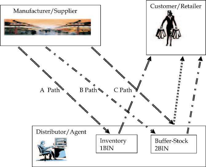
Path A: Order received at v(t) < u. Path B: Order received at w(t) > u. Path C: Order received exactly at u.

• Fig. 1: Logistic Diagram of the Model