An Exploratory Analysis between the Feature Selection Algorithms IGMBD and IGChiMerge

Published Online July 2017 in MECS

The ability of the Feature Selection (FS) process is to select the subset of prominent features and eliminate the features which provide little or no information for the prediction of class without distressing the performance of the classifier. It is also known as variable selection, variable subset selection, feature reduction or attribute selection. The benefits of feature selection are dimensionality reduction, better data visualization and understanding, storage reduction, speeding up the training and inference process and enhancing the model generalization. Because of these benefits now-a-days FS becomes an essential process in knowledge discovery. There are three major categories of models in subset selection. They are filters, wrappers and embedded model. Filters work independent of the predictor or classifier. The wrapper model uses the specific learning algorithm itself to assess the quality of the selected features. The embedded model performs variable selection in the process of training and is usually specific to given learning algorithms [18].

Discretization is a process which splits the range of continuous values into a small intervals and mapping each interval with a discrete symbol so as to provide useful information about the classes [12]. The discretization methods have been developed along different lines to meet different needs: supervised vs. unsupervised, splitting (top-down) vs. merging (bottom-up), dynamic vs. static, global vs. local and direct vs. incremental. The supervised discretization method is more accurate because it uses the class information for discretization, whereas the unsupervised discretization does not use the class information but it is fast. The topdown discretization method starts with an empty list of cut-points and keeps on adding by splitting intervals whereas the bottom up method starts with the full list of all the continuous values of the feature as cut-points and gradually removes by merging the intervals. A dynamic discretization would discretize when the classifier is being built whereas the static discretization is carried out prior to the classification task. A local discretization would perform discretization in a localized region of instance space but a global method uses the entire instance space. Direct discretization divides the range of continuous attribute into k -interval simultaneously and the value of k should be given by the user. The incremental method begins with simple discretization followed by an improvement process until stopping criteria is met [13].

The discretization process consists of four steps: i) sort the continuous values of a feature to be discretized ii) evaluate the cut-point for splitting or adjacent interval for merging iii) based on some criteria split or merge intervals of continuous values and iv) finally stop discretization [13].

The authors Mani.K and Kalpna.P (2015) have developed a novel FS method using Information Gain with Median Based Discretization ( IG MBD ) which is an unsupervised discretization method and proved that it provides better accuracy for Naive Bayesian Classifier ( NBC ) for the selected features. It has also been proved that IG MBD selects more relevant features than IG with Equal Width Interval Discretization ( IG_EWID ), IG with

Equal Frequency Interval Discretization ( IG EFID ) and IG with Cluster Based Discretization ( IG_CBD ) because the accuracy of the selected features using IG_MBD is more than that of the others.

It is noted that the unsupervised discretization methods are usually faster but not normally efficient than supervised discretization (Jerzy W. Grzymala-Busse, 2013). Thus this paper performs a comparative analysis between IG MBD , an unsupervised discretization method and Information Gain with ChiMerge discretization ( IG ChiMerge ), a supervised discretization method to determine which method provides better predictive accuracy for the NBC .

The rest of the paper is organized as follows. Section 2 depicts the related works. Section 3 describes the mathematical background required to understand the proposed methodology. The classification technique being used in this paper for prediction is presented in Section 4. Section 5 describes the comparison of IG MBD and IG ChiMerge . The results are analyzed in section 5. Finally section 6 ends with conclusion.

• II.    Related Works

An important issue related to mining large datasets both in dimension and size is of selecting a subset of original features using FS and this section provides an overview of several FS algorithms proposed in the literature.

Rajashree Dash et al, (2011) have discussed the basic concepts of discretization and different types of traditional supervised and unsupervised discretization techniques with examples. It was proved that an unsupervised method using k-means clustering gives equal performance as that of supervised methods viz., entropy based and chi-squared method [1]. James Dougherty et al, (1995) the authors compared the binning discretization methods with entropy-based and purity-based discretization methods. It was found that the performance of the Naive Bayes classifier is more using entropy-based discretization and proved that the discretized version of Naive Bayes algorithm slightly outperforms than C4.5. It was also observed that in some cases the performance of the C4.5 is significantly improved if the features are discretized in advance [3].

Ke wang et al. (1997) have proposed a minimum splits based discretization for continuous features to minimize the number of intervals with respect to impurity and proved that the proposed method generates a better decision tree [4]. The authors Salvador Garcia and et.al, (2013) have surveyed the discretization methods from the theoretical and empirical perspective. They tested the newest discretization methods using different types of classifiers for different datasets using different measures viz., accuracy, number of intervals and inconsistency [5]. Randy Kerber has described the ChiMerge, a general robust algorithm for discretization along with examples [6]. Arezoo Aghaei Chadegani and Davood Poursina (2013) have examined the of number of states for which the continuous variables are discretized will have the effect in the performance of Naive Bayes model and found that it provides best performance when the continuous variables are discretized into four states. It has also been identified that the performance deteriorates, when the number of states is increased to five or more [7].

The authors Derex D.Rucker et al, (2015) have showed that dichotomizing continuous variables via median based split and analyzing the resulting data via ANOVA involves a large number of costs and suggested to preserve the continuous nature of the variable and analyzing the data via linear regression [8]. A novel discretization method has been proposed by Daniela Joiţa (2010) based on k-means clustering algorithm which avoids the time required for the sorting the data items [10]. Jerzy W. Grzymala-Busse (2013) has launched entropy driven methodology for discretization with two enhancement options viz., dominant attribute and multiple scanning. They compared the proposed work with the well-known discretization methods viz., Equal Interval Width and Equal Frequency per Interval and proved that the entropy with multiple scanning is significantly better than the others [13].

Ying Yang and Geoffrey I. Webb (2002) have evaluated the effect of Naive Bayesian Classifier with nine discretization methods such as Equal Width Discretization (EWD), Equal Frequency Discretization (EFD), Entropy Minimization Discretization (EMD), Fuzzy Discretization (FD), Iterative Discretization (ID), Proportional K-interval Discretization (PKID), Lazy Discretization (LD), Non Disjoint Discretization (NDD) and Weighted Proportional K-interval Discretization (WPKID). It was found that the Naive Bayes Classifier with LD, NDD and WPKID achieves lower classification errors than of the others [14].

Nuntawut Kaoungku et al, (2013) have introduced a framework for missing value imputation and numerical data discretization using chi2 algorithm for classification and association rule mining and proved that the framework provides better results for both classification and association rule mining [15]. Prachya Pongaksorn et al. (2009) have designed a method for discretization called DCR, which uses both class information and the order between attributes to determine the discretization scheme with minimum number of intervals. They compared the DCR with five state of the art algorithms including two unsupervised and three supervised algorithms viz., EWID, EFID, CAIM, ChiMerge and WEKA discretization algorithm and proved that DCR requires fewer intervals, lower run time and provides high predictive accuracy than others [16].

K.Mani and P.Kalpana (2016) have developed a novel FS method using Bayes Theorem, Self Information and Sequential Forward Selection which uses the Median Based Discretization method for discretizing the continuous attributes into discrete and proved that their proposed work enhances the predictive accuracy for NBC [17].

From the existing literature it has been identified that many authors have introduced various novel methods for discretization and compared the same with the existing supervised and/or unsupervised discretization methods. In [2], the authors K.Mani and P.Kalpana (2015) have introduced a FS method called IGMBD and compared the same with three unsupervised discretization methods viz., EWID, EFID and CBD but they have not compared the same with any of the supervised discretization methods. Thus there is a need to compare the IGMBD with IGChiMerge and to verify the efficiency of the proposed work. Thus this paper performs the comparative analysis between IGMBD and IGChiMerge.

• III.    Mathematical Background

This section describes the mathematical background required to understand the methodologies compared in this paper.

• A.    Information Gain (IG)

It is a univariate, entropy-based and symmetric FS method based on Claude Shannon on information theory and it determines the feature relevance between the attribute and class label in a supervised way (Lei Yu and Huan Liu, 2003).

The entropy of X is computed as

H (X) = -E P (xi )log2( P (Xi))

The entropy of X after observing Y is computed as

H(X I Y) = -E P(yj)EP(xi | yj) log2(P(Xi I yj))

Where P(x_i) is the prior probability of all values of X and P(x i |y i ) is the posterior probability of X given Y . Thus the IG for a feature X and the class label Y is calculated as

IG(X | Y) = H(X) - H(X | Y)

Where H(X) is the entropy of X and H(X|Y) is the entropy of Y after observing X .

• B.    Pearson Chi-Square Test

It is used to determine the significant between the attributes A and B. Let ( A i , B j ) denotes the joint event that attribute A and B takes on value a i and b j respectively. Then the χ² is computed as

* ² =EEE; = 1

⁽ o ij - e ij )² e ij

Where oij and eij are the observed and expected frequencies of the joint event (Ai, Bj) respectively and it is computed as count(A = a.) x count(B = b .)

^ea =------------ i---------------j (5)

ijn

Where n is the number of data tuples, count ( A = a i ) and count ( B = b j ) is the number of tuples having value a_i for A and b j for B respectively. The χ2 statistic tests the null hypothesis (H 0 ) that A and B are independent with the significance level α = 1% and (r-1) × (c-1) degrees of freedom, where r and c are the number of rows and columns in the contingency table respectively. If the computed χ2 value is greater than the tabulated value then H 0 is accepted which means that A and B are correlated.

• C.    ChiMerge Discretization

It is a supervised discretization method based on χ² test. It employs a bottom-up approach by finding the best neighboring intervals and then merging them to form larger intervals recursively. Initially, each distinct value of numeric attribute A is considered to be one interval and χ² tests are performed for every pair of adjacent intervals. Adjacent intervals with at least χ² values are merged together, because low χ² values for the pair indicates similar class distributions. This merging process continues recursively until a predefined stopping criterion is met.

• D.    Computation of Median

Median is a measure of central tendency, which exactly splits the data into two halves. There are several ways for computing median. This paper uses the median computation method used in discrete frequency distribution. i.e., it considers the item which has the value ≥ (N+1)/2 , where N = ∑f as median.

• IV.    Classification Technique

There are three essential steps in the classification process. They are Model Construction (Learning), Model Evaluation (Testing) and Model Use (Classification). In the first phase, learning is performed on training data, which associates the class information and the classifier is built. In the second phase, the predictive accuracy of the model is computed based on test data. The percentage of test tuples that are classified correctly by the classifier from the test data becomes the accuracy of the classifier and the final step is used to classify the new instances [11].

• A. Naive Bayesian Classifier

  It is a statistical classifier based on the Bayes theorem. Let D be a set of training tuples with class label. Suppose there are m classes, C 1 , C 2 ,…,C m . The role of this classifier is to predict that the given tuple X belongs to the class having the highest posterior probability contained on X (H. Liu et al, 2002) . i.e., the tuple X belongs to C i iff P ( C | X ) >  P ( C | X ) for 1 <  j < m and j + i . P ( C i | X ) is computed as

P ( Ci | X ) =

P ( X | C_i ) P ( C_i ) P ( X )

The accuracy of a classification method in general is the percentage of records that are classified correctly by the classifier in the test data and is computed as

TP + TN Accuracy =----------------

TP + TN + FP + FN

Where True Positive (TP) refers to positive tuples that were correctly identified by the classifier, True Negative (TN) refers to negatives tuples that are correctly identified by the classifier, False Positive (FP) refers to negative tuples that are incorrectly classified and False Negative (FN) refers to positive tuples that were incorrectly labeled by the classifier (Jiawei Han, Jian Pei, and Micheline Kambar, 2011).

• V.    Comparison of Median Based Discretized IG and Chimerge Discrtized IG

The objective of the paper is to compare two FS methods viz., IG MBD and IG ChiMerge . The MBD is an unsupervised, global, static and incremental method which uses splitting for discretization where as ChiMerge is a supervised, global, static and direct method which uses merging process for discretization. IG is one of the popular measures used in FS . For continuous attributes the IG considers the split which gives high IG as the best split and it takes considerable among of time to find IG . The IG MBD uses median ( M ) based discretized values for continuous features. I.e., it uses M as the measure to split the continuous attributes into two halves and converts them into discrete based on M . It is an un-supervised discretization scheme and the corresponding pseudo code is shown below

Pseudo Code 1 (PC1): Computation of MBD

• 1.    for each continuous attribute F i in the training set S do

• i.    compute median M ;

• a)  sort the values of a continuous feature F i in

ascending order;

• b)  for each unique value x i in F i , calculate the

frequency of occurrence f and cumulative frequency cf ;

• c)    Mid ← (N+1) / 2 where N = ∑f ;

• d)    M ← the item which has cf ≥ Mid;

• ii.    perform discretization

• a)    F i_des ←{low,high} ;

• b)    for each x i ∈ F i

if x i >  M then x i ← F i_des [1] ;

else x i ← F i des [0] ;

The main advantage of MBD is that there is no need to specify the number of intervals because it splits the range of the continuous values into two halves and also there is no possibility for outliers. IG_ChiMerge uses ChiMerge discretized values for continuous features and its pseudo code is shown below.

Pseudo Code 2 (PC2): ChiMerge Discretization

• 1.    for each continuous attribute F i in the training set S do

• i.    no_of_interval ← number of distinct values in F_i

• ii.    place each distinct value of F i in one interval iii. compute χ² test for each adjacent intervals

• iv.    merge the adjacent intervals with least χ² values

• v.    no_of_mer_int ← number of intervals merged

• vi.    no_of_interval ← no_of_interval - no_of_mer_int

• vii.    repeat from step 1(iii) until stopping criteria

• viii.    perform discretization

• a)    k←no_of_interval

• b)    F i_des ={ d_v 1 ,d_v 2 ,...,d_v k }

• c)    assign d_v i for the values in the interval i,1≤i≤k

The discretized datasets obtained using both methods are then fed into IG, which computes the expected information for each attribute. The attributes are ranked based on their respective IG 's. From the ranked attributes the a ttributes whose IG is greater than the threshold are selected as the more relevant attributes where the threshold is fixed as M of the IG' s computed. The selected features of both methods are fed into the NBC to determine the predictive accuracy.

• A.    IG MBD : An Example

In order to understand the relevance of the method IG MBD , the weather dataset has been taken from the UCI machine learning repository and it is shown in Table 1.

Table 1. Weather dataset

Outlook	Temperature	Humidity	Windy	Play
Sunny	85	85	FALSE	No
Sunny	80	90	TRUE	No
Overcast	83	86	FALSE	Yes
Rainy	70	96	FALSE	Yes
Rainy	68	80	FALSE	Yes
Rainy	65	70	TRUE	No
Overcast	64	65	TRUE	Yes
Sunny	72	95	FALSE	No
Sunny	69	70	FALSE	Yes
Rainy	75	80	FALSE	Yes
Sunny	75	70	TRUE	Yes
Overcast	72	90	TRUE	Yes
Overcast	81	75	FALSE	Yes
Rainy	71	91	TRUE	No

Table 2. Frequency and cumulative frequency for each unique values of temperature attribute

Unique values of Temperature	Frequency of occurrence ( f )	Cumulative frequency ( cf )
64	1	1
65	1	2
68	1	3
69	1	4
70	1	5
71	1	6
72	2	8
75	1	10
80	1	11
81	1	12
83	1	13
85	1	14

The dataset contains 5 fields viz., outlook, temperature, humidity, windy and play. Among these attributes, the temperature and humidity contain continuous values. As specified in PC1, the frequency (f) and cumulative frequencies (cf) of each sorted unique values (xi) of temperature attribute are computed and it is shown in Table 2.

From Table 2, Mid = (14+1)/2=7.5 and hence M =72. Based on the M the temperature is discretized as {high, high, high, low, low, low, low, low, low, high, high, low, high, low }. Similar procedure is applied to other continuous features too and the discretized values are shown in Table 3.

Table 3. Discretized values of continuous attributes in Weather dataset after MBD

Temperature	high, high, high, low, low, low, low, low, low, high, high, low, high, low
Humidity	high, high, high, high, low, low, low, high, low, low, low, high, low, high

After discretization the IG is computed for all attributes. The entropy of play, H(Play) is -(9/14 × log 2 (9/14) + 5/14 × log 2 (5/14)) = 0.94028. The outlook feature contains 3 unique values viz., overcast, rainy and sunny. 4 instances of outlook contain overcast as its value. Out of these, all 4 instances have the value 'yes' for play attribute. Similarly 5 instances of outlook attribute contain the value 'rainy' and 'sunny' each. Out of the 5 rainy instances 3 contain 'yes' and 2 contain 'no' for play. Similarly out of the 5 sunny instances 2 contain 'yes' and 3 contain 'no' for play. Therefore the expected information needed to classify a tuple in weather dataset, if the tuples are partitioned according to outlook is

H(Outlook|play) =(4/14 × (-(4/4 × log 2 (4/4)))) + (5/14 × (-(3/5 × log 2 (3/5) + 2/5 × log 2 (2/5)))) + (5/14 × (-(2/5 × log 2 (2/5) + 3/5 × log 2 (3/5) ))) = 0.69354

Therefore, IG (Outlook|Play) = 0.94028-0.64353

= 0.24675 using (3).

Similar calculations are to be performed for other attributes too and the final ranking for the weather dataset is shown in Table 4. From the ranked attributes outlook and humidity are selected as the more relevant features because their IG 's are greater than 0.0999, where 0.0999 is the threshold, which is the median of the IG' s in Table 4.

Table 4. Feature Ranking by IG with MBD

Feature (F i )	IG(F i ) after MBD
Outlook	0.2468
Humidity	0.1518
Windy	0.0481
Temperature	0.0013

• B.    IG_ChiMerge : An Example

Using chi-square test the critical values for the first two intervals of the feature temperature is shown in Table 5.

Table 5. Contingency Matrix

Interval	Play		Total
	Yes	No
I	1(0.5)	0(0.5)	1
II	0(0.5)	1(0.5)	1
Total	1	1	2

From table 5, o₁₁= 1 , o₁₂= 0 , o₂₁= 0 and o₂₂= 1, e ₁₁= (1×1)/2 = 0.5, e 12 = (1×1)/2=0.5, e 21 = (1×1)/2=0.5 and e 22 = (1 x1)/2=0.5 and the / 2 statistics is calculated as

/ 2 = (1-0.5)²/ 0.5 + (0-0.5)²/ 0.5 + (0-0.5)²/ 0.5 + (1-0.5) / 0.5 = 2.

The table / 20.01,1 = 6.63 5. Since the calculated / 2 (2) < the table value (6.635), the intervals are merged. Similar computation is performed for other adjacent pair of intervals and they are shown in Table 6.

Table 6. Demonstration of ChiMerge Discretization

Original temperature values	85	80	83	70	68	65	64	72	69	75	75	72	81	71
Sorted Temperature	64	65	68	69	70	71	72	72	75	75	80	81	83	85
Play values	V	n	У	У	У	n	n	У	V	у	n	V	V	V
Initial Interval	64	65	68 69 70			71 72		72 75 75			80	81 83		85
Calculated y2	X2=2 ^=4          /2-5      ^«5          -^=4 /2-3      /2.3
Merged content after 1st iteration	64 65		68 69 70			71 72		72 75 75			80	81 83		85
Calculated y2	/2=1.875        x2-5     x2*5           ^*4 x2*3      x2-3
Merged content after 2ad iteration	64 65 68 69 70					71 72		72 75 75			80	81 83		85
Chi square	X;”3 733 xz-5          Z2-4/2-3     Zz-3
Merged content after 3fd iteration	64 65 68 69 70					71 72		72 75 75			80 81 83   85
Chi square	X2-3.733   z2*5          Z2=										2.1
Merged content after 4th iteration	64 65 68 69 70					71 72		72 75 75 80 81 83 85
Chi square	Z2=3.733 Z2=3.214
Merged content after 5 th iteration	64 65 68 69 70					71 72 72   75 75 80 81 83   85
Chi square	/М.836543
Merged content after 6th iteration	64 65 68 69 70 71 72 72   75 75 80 81 83   85

After finding the critical values, the first two intervals are merged together because it has least χ² value. This process is repeated until the calculated χ² value is greater than 6.635 or when all items of a feature fall in the same interval. From table 5, it is observed that after 6 iterations, all values of temperature fall in one interval and it is discretized as [ true, true, true, true, true, true, true, true, true, true, true, true, true, true ]. Similar procedure is applied to other continuous attributes too and the discretized values of the continuous attributes temperature and humidity of weather dataset after

ChiMerge discretization is shown in Table 7.

Table 7. Discretized values of continuous attributes in Weather dataset after ChiMerge discretization

Temperature	high, high, high, high, high, high, high, high, high, high, high, high, high, high
Humidity	high, high, high, high, high, high, high, high, high, high, high, high, high, high

After discretization, the IG is computed for the discretized dataset as in section 5(A) and the ranking are shown in Table 8.

Table 8. Feature Ranking by IG ChiMerge

Feature (F i )	IG(F i ) after ChiMerge
Outlook	0.2468
Windy	0.0481
Humidity	0.0000
Temperature	0.0000

The attributes outlook and windy are selected from the ranked attributes as the more relevant feature because their IG 's are greater than 0.0241.

• VI.    Experimental Study

In order to analyze the said methods, 6 datasets have been taken from UCI Machine Learning Repository [9]. Each dataset contains both continuous and nominal features. The missing values for each attribute in the datasets are filled with their corresponding mean. The detailed specification of these datasets is shown in Table 9.

IG MBD and IG ChiMerge discretization are fed into the NBC and accuracies are computed using WEKA tool with 10fold cross validation technique. The results are shown in Table 10.

Table 10. Comparison of Predictive Accuracy of NBC for the selected features using IG ChiMerge and IG MBD

Dataset	#Selected features	Accuracy (%) of NBC with
		All Features	Selected Features using
			IG ChiMerge	IG MBD
Pima Indian Diabetes	4	76.3021	75.3906	76.5625
Breast cancer	5	95.9943	95.9943	95.2790
Statlog heart	6	83.7037	85.1852	85.1852
Eeg	7	48.0406	52.2131	48.9285
Weather	2	64.2857	57.1429	71.4286
Ann-train	10	95.6522	95.5992	95.7317
Average		77.3298	76.9209	78.8526

The number of original features and the selected features of both methods are shown in Figure 1. Since median IG' s is fixed as threshold, both methods select the same number of attributes approximately 50%. Figure 2 shows the accuracy comparison of NBC with all features, selected features with IG MBD and IG ChiMerge .

Table 9. Description of the datasets

Dataset	No. of Attributes	No. of Instances	No. of Classes
Pima Indian Diabetes	9	768	2
Breast Cancer	11	699	2
Statlog Heart	14	270	2
Eeg	15	14979	2
Weather	5	14	2
Ann-train	22	3772	3

The IG MBD has been implemented in Python, ChiMerge discretization is obtained using chiM function of ' discretization ' package in R tool and IG is using WEKA tool. The original features and the selected features using

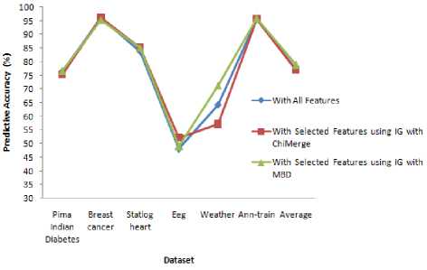
Fig.2. Comparison of predictive accuracy of NBC with all features and with selected features using IG MBD and IG ChiMerge

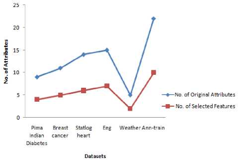
Fig.1. Comparison of number of original features selected features using IG MBD and IG ChiMerge

From table 10, it is observed that, the accuracy of Pima Indian Diabetes, Weather and Ann-train is greater using the selected features with IG_MBD . Similarly the accuracy of Breast cancer and Eeg, the accuracy of NBC has greater value for the selected features with IG_ChiMerge . The accuracy of Statlog heart remains the same for both methods. It is observed that the accuracy of the selected features using IG MBD is 78.8526% on an average which is greater than the selected features using IG ChiMerge (76.9209%) and also with original features (77.3298%).

This is because MBD uses median which is one of the measure of central tendency and it splits the continuous attributes into two halves which ultimately leads no two values fall in the same group where as the ChiMerge discretizes uses ' n ' iterations, each comprising of chisquare test and merging intervals. It is noted that a minimum number of discrete intervals reduce the data size which results in better understanding of the discretized attributes. IG MBD has two intervals where as IG ChiMerge has ' i ' intervals where 1 ≤ i ≤ n and ' n ' is the maximum number of intervals. As IG MBD has only two intervals and provides more accuracy than IG ChiMerge, , it is proved that IG MBD is better than IG ChiMerge .

• VII.    Conclusion

  This paper compares IG MBD with IG ChiMerge by measuring the accuracy of NBC on several different datasets. It is evident from the table that the accuracy of the NBC using IG_MBD is increased by 1.9317% on an average when compared with IG ChiMerge . It is also proved that for the reduced feature set, there is an accuracy enhancement of 1.5228% than the original features. The result clearly shows that the model constructed using IG MBD performs well for NBC and is equally competent with IG ChiMerge . Further both methods reduce the features by 50% which reduces the classification time and the space requirements too.