An Heuristic Approach to Solving the one-to-one Pickup and Delivery Problem with Three-dimensional Loading Constraints

Author: Rémy Dupas, Igor Grebennik, Oleksandr Lytvynenko, Oleksij Baranov
Journal: International Journal of Information Technology and Computer Science(IJITCS) @ijitcs
Article in issue: 10 Vol. 9, 2017.
Free access
A mathematical model and a solving strategy for the Pickup and Delivery Problem with three-dimensional loading constraints regarding a combinatorial configuration instead of a traditional approach that utilizes Boolean variables is proposed. A traditional one-to-one Pickup and Delivery Problem in a combination with a problem of packing transported items into vehicles by means of the proposed combinatorial generation algorithm is solved.
Pickup and Delivery problem, vehicle routing, 3D loading constraints, combinatorial configuration, generation, packing of parallelepipeds
Short address: https://sciup.org/15012686
IDR: 15012686
Text of the scientific article An Heuristic Approach to Solving the one-to-one Pickup and Delivery Problem with Three-dimensional Loading Constraints
Published Online October 2017 in MECS
A vehicle routing problem (VRP) plays an important role in the logistics management. A wide variety of the vehicle routing problems has been studied lately [1-3]. Different classes of the vehicle routing problem describe various practical situations, but they are mostly focused on a common problem – an efficient use of a set of vehicles that must serve customers’ orders.
In addition to routing vehicles, real-world transportation companies also require solving a problem of loading vehicles which means that it is not sufficient enough only to decide how to route vehicles, but also how to load cargos to them. Such an integrated problem was introduced in [4] for the first time and it was called as the “capacitated vehicle routing problem” (CVRP) with three-dimensional (3D) loading constraints (3L-CVRP). In 3L-CVRP, every customer requires transporting one or a few parallelepipeds (or boxes) where each one is represented by a 3D rectangular loading space and its weight (in contrast to the traditional
CVRP, where an only weight is given). Surveys [5] and [6] show a recent state of the art for solving the integrated vehicle routing and loading problems.
One of the most popular VRP models is the Pickup and Delivery Problem (PDP) [7-10], where every customer has to pick up some item/items at one location and to deliver it/them to another location. The Pickup and Delivery Problem arises naturally in several contexts such as urban courier services and door-to-door transportation systems [11].
The Pickup and Delivery Problem (PDP) is about routing a set of vehicles in order to serve a set of transportation requests between given origins (pickup points) and destinations (delivery points). Every route should start and finish at a pre-defined depot and satisfy pairing and precedence constraints: the origin (a pickup point) should precede the destination (a delivery point), and every pickup-delivery pair should be visited by the same vehicle [11]. There are a lot of additional constraints on PDP such as time windows [7, 12], time constraints related to vehicles availability [10], etc.
A lot of heuristics and metaheuristics were used for solving PDP: the reactive tabu search [13], the tabu embedded simulated annealing [14], the squeaky wheel optimization [15], the grouping genetic algorithm [16], the construction heuristic [17], the hybrid algorithm (the simulated annealing and the large neighborhood search) [18], the adaptive large neighborhood search, the indirect local search with greedy decoding [19], and the guided ejection search [20] etc.
In case of the vehicle routing problem, solving the Pickup and Delivery Problems in the real-world applications also demands taking the loading constraints into account. Articles which solve PDP consider such constraints as LIFO [21] or FIFO [22] buffers, or as the 2D or 3D loading constraints [23-26].
Despite a wide variety of articles dedicated to PDP, it is hard or impossible to regulate a balance between a solution time and a result’s precision in most of the solution algorithms. An objective function and all limitations in PDP are usually described as inequalities with the help of Boolean variables.
In this article, a mathematical model for the Pickup and Delivery Problem with the 3D loading constraints which utilizes combinatorial sets instead of commonly used Boolean variables is provided. The combinatorial generation algorithm for solving the described problem is also given. An advantage of the described algorithm is its ability to balance between the quality and the time of solution. The Given solution algorithm produces quite good results in a reasonable time.
The paper is organized as follows. Section II describes a mathematical model. Section III gives basic details of the decision strategy. Section IV demonstrates the solution algorithm for a lower level. Section V gives explanations to computational experiments. Conclusions are given in Section VI.
-
II. The Mathematical Model
-
A. The problem formulation
We are considering the traditional Pickup and Delivery Problem (PDP) [27], one-to-one, a symmetric case, i.e. every arc ( i , j ) is equal to the arc ( j , i ) and can be replaced by one edge. The Pickup and Delivery Problem is modeled on a complete graph G = (V , A) where V is a set of all vertices, V = {0,1,...,2 n + 1} , where 0 and 2 n + 1 denote a depot and A is a set of all the arcs.
There are v identical vehicles available; each vehicle has a loading space in the form of a parallelepiped (defined by a width W , a height H and a length L ) and a weight capacity Q . Every transportation request i e Jn , Jn = {1,2,..., n } requires the pickup or delivery of one three-dimensional item having a width wi , a height hi and a length li with a total weight qi ( qi is positive for pickups and is negative for delivery points). We assume that all the items are rectangular boxes .
There are some constraints on the loading items of a vehicle (the 3D constraints ):
-
1. Inside a vehicle, the items can only be placed orthogonally; however, they can be rotated by 90 ° in the width–length plane.
-
2. The stability constraint: every transported item should be placed on a vehicle’s floor; it can be also placed on top of another item. In such case, the item should be completely supported by the one below, i.e. we do not allow any part of the item to be in limbo.
-
3. The blocking constraint: we should ensure that items can be easily unloaded in their delivery point which means that when a delivery point is visited,
two conditions should be satisfied:
-
• an item to be unloaded should not be stacked beneath other items in the vehicle. An item A is beneath an item B if the interior of the projections of their bases to the vehicle’s floor intersects, and the top of A is not higher than the bottom of B in a vertical direction;
-
• the unloaded item should not also be blocked by other clients’ items that will be visited later. The item is also blocked if it overlaps any item of a next client when it is moved along the L axis towards a rear door.
The objective is to find a set of at most v routes (one per a vehicle) such as:
-
1. Every route begins at the depot and after all clients have been visited ends at the depot.
-
2. Every client (i.e. a pair of pickup and delivery points) is served by the same vehicle.
-
3. A total weight of transported items does not exceed a vehicle’s capacity.
-
4. Items are packed in a vehicle according to the 3D constraints.
-
5. A total cost of all routes is minimized.
-
B. Designations
P denotes a set of pickup vertexes, P = {1,2,..., n } ;
D signifies a set of delivery vertexes, D = { n + 1, n + 2,...,2 n } ;
-
qi marks a vehicle’s load at the vertex i ; qi is positive at pickup nodes i = {1,2,..., n }; it is negative at delivery nodes i = { n + 1, n + 2,..., 2 n } ;
-
wi , hi , li signify orthogonal dimensions (a width, a height and a length) of the item at the vertex i , i e J 2 n ;
-
v is a number of vehicles;
Q determines a capacity of a single vehicle (all vehicles have the same capacity);
W , H , L are orthogonal dimensions (a width, a height and a length) of every loading space respectively,
C stands for a set of the pickup-delivery pairs, C = {( P i , d i )} , P i e P , d i e D , d i = P i + n , i e J n ;
CvC 2,..., C v define a partition of C : C = (J C j , j = 1
C i n C j = 0 , i e J v , j e J v ; each subset C j corresponds to a vehicle j that serves this set of clients, j e J v ,
v nj = Card Cj , j e Jv , ^ nj = n ;
j = 1
c ( i , j ) is a cost of a traversing edge ( i , j ) ;
Vj = {i(,ij,...,ij } is a set of all pickup and delivery points included into Cj ;
P ( Vj ) stands for a set of permutations of elements from Vj that describes all possible paths of the vehicle j ;
Q ( ij ) denotes a current load of the vehicle j at a moment of arrival to the vertex i j , k e J 2 n . ;
u j = ( x j , y j , z j ) determines coordinates of a pole of the placement area in the vehicle j .
-
C. Decision variables of the problem
U = (U 1,U2,...,Uц), Uj = (u,uj,...,uj ) where 12 nj uj = (xj, yj, zj ) stands for coordinates of the pole of the item i in the vehicle j ;
П e P(V j ) is a route of the vehicle j;
vJ i = ( lw i , h i ), lw i e {( l i , w i ),( w i ,l i )} marks orientation of the item i in the vehicle j , i e V j , j e J ^ .
For n transported items
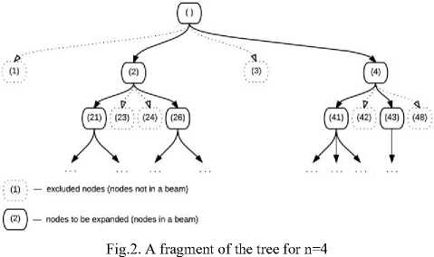
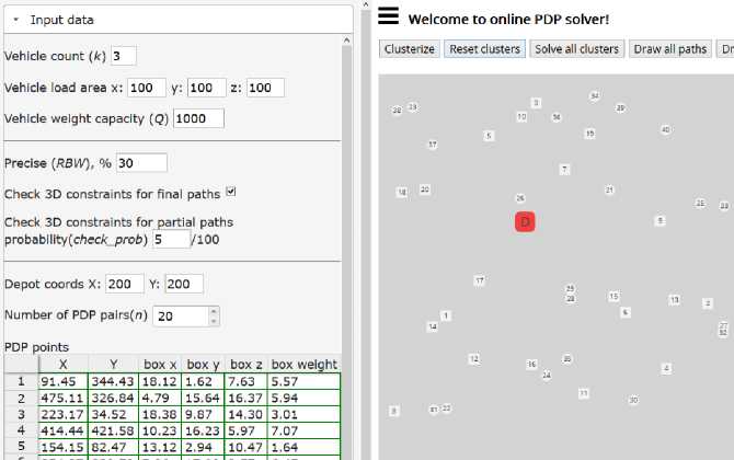
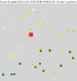
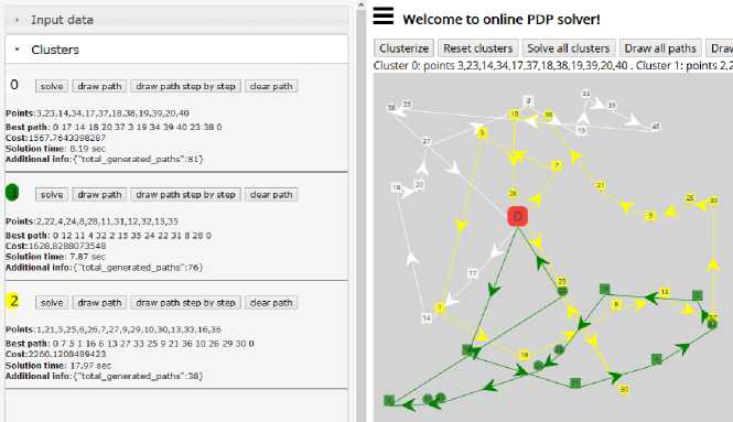
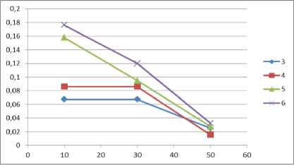
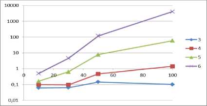
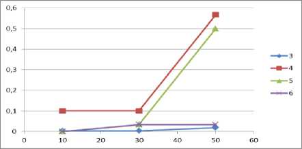
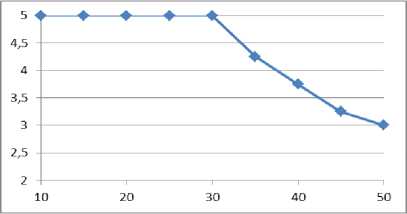
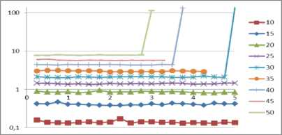
Пi = {x eR :x = (xi,x2,Хз)|0 Dj = {x e R3 : x = (xi,x2,X3) |0 < xi < L, 0 < x2 < W ,0 < x3 < H}. D. Φ-functions Ф -functions [28] make it possible to describe formally conditions of the mutual non-intersection for two parallelepipeds and the condition for correct placement of parallelepipeds in a placement area [29]. To describe the 3D constraints, we use two Ф -functions: Ф°(uj, uJm, vj, vJm ) is used for checking that the item i (which is determined by coordinates of a pole u j and an orientation v j ) does not intersect with an item m (which is determined by coordinates of a pole umj and an orientation vmj ); Фjm (uj, um, vJm ) is used for checking that the item m can be correctly placed into the placement area Dj (which is determined by W (a width), H (a height) and L (a length) of the vehicle’s loading space). фj(uj,um,vj,vJm) = max{xJm—xi -vii, — xm + xi— vi m, ym— yi— v2 i,— ym+ yi— v2 m, zm zi v3 i, zm+zi v3 m}; фJjm (u0 ,um, vJm ) = min{xJm — x0,— xJm + x0 + L — vim, ym — y 0,— ym + y 0 + W — v2 m, zm — z0, —zm+ z0 +H— v3 m}. If Фjim (uj, uJm, vj, vJm) > 0 for all i, m e Jn, i< m , then there’s no intersecting pair of items in a vehicle. If Ф0m (uj, uJm, vJm ) > 0 for all m e Jn , then each item is placed correctly inside the vehicle’s loading area. Thus, items’ placement in vehicles should be performed in such a way that the described Φ-functions are positive. E. An objective function and constraints ц . 2ni —1 .. Z[c(0,ii')+ Z c(ik,iJk +i)+c(i-jn.,2n+i)]^min; .j=i k=i Q(ikj) = ZZf (ij) < Q , v5 e J2 , j e J^ ;(2) k=i f (i) = qi, —%, if i<= n (a vertex is a pickup); if i > n (a vertex is a delivery); ф im (uj , um, vi , vJm ) > 0, i,m e Jn, i < m,. 1 . , j e J^(3) _Ф()m(u0 , uJm, vJm ) > 0, m e Jn, Here c(0, ij) is a distance between the depot (a fictive vertex 0) and the first vertex visited by the vehicle j; c(ij ,2n +1) is a distance between the last visited vertex and the depot (a fictive vertex 2n+1). It should be noted that the fictive vertexes 0 and 2n+1 designate the same depot. III. The Decision Strategy We propose a two-level strategy for solving the problem. A. An upper level - partitioning In the upper level, we are splitying a set C into subsets (clusters) C1,C2,...,Cv . Each cluster Cj contains pickup-delivery pairs (pi, di) which are served by the vehicle j. For solving the clustering [30] problem, we chose the simplest k-means algorithm [31-33]. The traditional k-means algorithm deals with single points, but we want to make clusters of pairs (pi,di) . We are substituting the pair ( pi, di) with a single point ki , which is a middle point between pi and di : ki. x = pi. x + di. x Pi. У+di. У where .x,. y are coordinates of the points. B. A lower level – path constructing In the lower level, we are constructing a route for the vehicle j for a single cluster Cj . As mentioned above, a permutation nj e P(Vj) describes a path of the vehicle j. The vehicle’s route defines an order of items’ loading and unloading to/from the vehicle j . Every path nj should meet all the constraints described in Section 2. To describe items’ rotations in the width-length plane, we substitute each element of nj (which is either a pickup point or a delivery one) by a vector lwi e {(li,wi-),(w,,li)} , i e Vj . This combinatorial permutation is called “a composition of permutations” [34]. So, to construct a route for the vehicle j, we should choose a permutation nj e P(Vj) so that it minimizes the objective function (1). The algorithm’s solution for this problem is described in the next section. IV. Solving the Algorithm for the Lower Level A. The exact solution To generate permutations nj , we use the GenBase algorithm [35]. It is universal and can be used for generating a wide variety of different combinatorial sets. Let us denote a path of the vehicle j as t = П ; let’s also call first i vertexes of a path t as a partial path ti = (t1,t2,..., ti). The GenBase algorithm is recursive: at every level i e J0n-1 , J2n-1 = {0,1...2n-1} , it adds a successive vertex ti+1 to the end of the current partial path tl= (t1,t2,..., ti) and obtains a new partial path ti+1= (t1,t2,...,ti+1) at the next level. At the level i=2n, the algorithm produces a full path t2n= t. Elements ti+ should meet the constraints specific to a particular combinatorial set. At every level i e J0n । , let us denote a tuple of all those elements as F = (/1, f2,..., fk) . So, for each j e Jk, Jk = {1,2...k}, the GenBase algorithm adds a new element ti+1 = fj to the current partial path ti = (t1,12,...,ti) and recursively calls itself with the new partial path ti+1 = (t1,12,..., fj ). To generate all the paths, the GenBase algorithm is called with an empty path t0= ( ) . function GenBase( ti ) { if i = 2n then {output = output иti; exit;} determine Fi ; for j = 1,2,...,| Fi | do GenBase(ti+1= (t1,12,...,ti, fj )); } For PDP paths, we have following constraints for a tuple Fi : 1) vertexes in ti aren’t duplicated ti+1 ^ tz, z = 1... i; 2) for every pickup-delivery pair, a vehicle should visit a pickup point before a corresponding delivery point: ti+1 > n —z :(ti+1 - n) = tz . For example, when n=4 (i.e. there are four pickupdelivery pairs), the delivery point 5 can be added to the path only if the corresponding pickup point 1 has already been added to the path; 3) the restriction (2) that limits the maximum vehicle’s load should be satisfied; 4) if ti+1 is a pickup, it means that a new item will be loaded into a vehicle, and we should check the 3Dconstraints. For this reason, the algorithm [29] should be used. It should be noted that the algorithm [29] has an ability to rotate every item in the width-length plane for the optimal packing. Thus, vectors lwi, i e Vj , are determined. The GenBase algorithm produces a recursive tree, where every node at intermediate levels i< 2n-1 is a partial path and nodes at the last level i = 2n-1 are full paths. At levels i< 2n-1, a tree node is expanded by adding a new node from Fi to a partial path. Example 1. Let’s demonstrate how GenBase works while generating paths for n=2 (the vertexes 1 and 2 are pickups, and the vertexes 3 and 4 are deliveries). At first, at the level i=0, F0 consists only of pickup vertexes F0= (1,2) . Each pickup is added to the end of a current empty path t0= ( ) making a new path (t1= (1) in the first case and t1= (2) in the second one). After that, GenBase is called recursively for each vertex t1. At the next level i =1, for the path t1= (1), it is possible to add either a pickup vertex 2 or a delivery vertex 3 corresponding to the pickup vertex 1. A vertex 4 can’t be added because there is no corresponding pickup vertex 2 in the current path t1= (1) . Fig.1. A recursive tree generated by the algorithm When all full paths have been generated by the algorithm (so we have the complete tree), a resulting path will be a path that owns the best value of the objective function (1). B. An heuristic solution A powerful beam search heuristic [36] can be applied to algorithms that produce recursion tree. The beam search heuristic is an adaptation of the branch and bound method where only some nodes are evaluated in the search tree [37]. At any level, promising nodes are only kept for further branching, and the rest of nodes are being pruned off permanently [37]. In terms of our problem, the beam search heuristic acts at the step of expanding tree nodes (i.e. extending partial paths with points from the set Fi ). In an original version, it takes some predefined amount of “best” points from Fi (a beam width) for further expanding and pruning off others. We slightly modified heuristic and made the beam width a relative value – some percent of tree nodes. We will call it a relative beam width (RBW). So, for our problem, the beam search heuristic can be applied as follows: H1. The algorithm sorts new points from Fi by ascending a distance: • from the depot, if i=0 (so, the first point in a route should be as close to the depot as possible); • a last node in the current path for all other cases. H2. The GenBase algorithm calls itself recursively only for the first RBW% of points from Fi (RBW is a predefined parameter). Other nodes are pruned off. H3. Since checking the 3D constraints is the NP-complexity task [29], they are checked not when a vehicle arrives to a pickup point, but time-by-time, with a probability check_prob e [0;1]. An only exception is the last level i=2n-1, where we always check the 3D constraints because it is necessary for the final path to meet them. The power of the described algorithm and the heuristic is that one can regulate a balance between a solution’s quality and the algorithm’s operating time by changing the RBW value. Example 2. Let us demonstrate how the heuristic works for n=4 (points 1-4 are pickups and points 5-8 are deliveries). Let’s set RBW=50% which means that we will expand each tree node with a half of points in Fi at all steps i<2n-1. At the beginning, at the level i=0, F0 consists of all pickup vertexes F0= (1,2,3,4) . We are sorting them by distances to the depot. Let’s assume that we obtain (2,4,3,1), and we take first two points (2 and 4) for further expanding. Points 1 and 3 are excluded from further consideration. The same idea works for the next levels as well. Let’s see what’s happening at the level 1 for a partial path t1= (2) . There’re four candidates: three other pickups (1,3 and 4) and a delivery point 6 corresponding to a pickup point 2 (6=2+n, n=4), so F1= (1,3,4,6) . Let’s suppose that the points 1 and 6 are the closest ones to the point 2, so we will expand them by skipping the points 3 and 4. So, here t2= (21) and t2= (26) . In Fig.2, one can see a fragment of the tree for n=4, where nodes that were present in Fi but later excluded are marked with dots. Issue 1. An attentive reader might observe that due to H3 at a penultimate level i = 2n-2, the heuristic can theoretically produce a path ti that doesn’t meet the 3Dconstraints (because H3 allows skipping a check of the 3D constraints). At the last level, we always check the 3D constraints (to prevent an output of an invalid path), it can be a situation when all paths or partial ones t2n-2 will be invalid (in terms of the 3D constraints) and only a final check at the last level i = 2n-1 will let us know that all the current partial paths are invalid. So, H3 can lead to a situation when the heuristic is not able to give a solution. An example of this situation is: we have such a small RBW value that only one tree node is expanded at each level (i.e., RBW=1%) and we also have a small check_prob value, so the 3D constraints are rarely checked. So, the algorithm can produce a partial path which doesn’t satisfy the 3D constraints and recognize it only when it performs a mandatory check of the 3D constraints on the full path. At that point, it can only be seen that the generated path was incorrect. The described situation can be avoided by increasing values of check_prob and RBW. In practice, it is usually enough to set a value of check_prob = 0.2 to avoid the described situation. V. Computational Experiments A. A program description We developed the program that solves the described problem and has a user-friendly interface. It is available online at http://pdp- Its demo can be found at Input parameters are: • The vehicle’s parameters: o a vehicle’s count (a number of clusters); o a load area and a weight capacity for every vehicle. • Parameters of a point: o coordinates of the depot; o a number of the pickup-delivery pairs; o coordinates of each point, a box weight and a size (for pickup points). • The solution’s parameters: o RBW,%; o trans_prob is an indicator that is intended to check the 3D loading constraints for full paths (if unchecked, and trans_prob is 0, the 3D constraints will not be checked, and the solution will be obtained quickly). The program can: 1) distribute all PDP pairs between vehicles (and form clusters); 2) obtain the heuristic solution described in Section 5.2 for each vehicle (cluster). B. Comparing the proposed algorithm with well-known ones The table below demonstrates results of computational experiments: we obtained a lot of generated paths and a cost of the best path through varying n and RBW (coordinates of the vertexes are generated randomly within the range 0…500). A load capacity, a width, a height and a length of the vehicle were set to huge values (so, the 3D constraints were always satisfied). The results are presented in a format like “a total count of generated paths”/ ”a length of the best route”. For example, the program generated 298 routes and a cost of the best path was 1869 for 2n=12 and RBW=20%. We compared the results with the well-known two-phase heuristic by Renauld [38] with parameters R=5 and various values of α: α=0.5; 1; 1.5 (Tables 1 and 2). We programmed the Renauld’s algorithm ourselves. It is worth mentioning that the Renauld’s approach does not take into account any loading limits. That is why we mitigated all the loading limits (we assigned large values to W, H, L and Q) while comparing our results with the Renauld’s ones. As one can see, while our approach is more complex and takes into account the vehicle’s loading, the results obtained aren’t much worth than the ones obtained by means of a two-phase heuristic. However, a serious disadvantage of our algorithm is its working time: while the Renauld’s algorithm is processing data only for a few milliseconds, our program can be processing data for a rather long period (up to 60 seconds for 25 PDP pairs). Fig.3. A screenshot with all input parameters and PDP points ► Input data ’• Clusters 0 solve draw path draw path step by step clear path Points:3,23,14,34,17,37,18,38,19,39,20,40 No path hasn't obtained for cluster yet "solve draw path draw path step by step clear path Points:2,22,4,24,8,28,11,31,12,32,15,35 No path hasn't obtained for cluster yet 2 solve draw path draw path step by step clear path Points: 1,21,5,25,6,26,7,27,9,29,10,30,13,33,16,36 No path hasn't obtained for cluster yet Welcome to online PDF solver! Clusterize | Reset clusters Solve all clusters Draw all paths] | Dra Fig.4. A screenshot of clustering 20 pickup-delivery pairs (squares are pickups and circles are deliveries; the big rounded red square is a depot) Fig.5. A screenshot of a generated path for each cluster from the example above Unfortunately, we could not find any articles (except [38]) with publicly accessible test instances that are devoted to the PDP problem with constraints similar to the ones we have considered. That is why we were comparing our results with the Ropke’s ones [39], which are shared at The Ropke’s work is devoted to the multi-vehicle PDP problem with time windows. A formulation of the Ropke’s problem also takes into account a capacity Q of every vehicle. While comparing results, we used the same Q value as in the Ropke’s samples. However, our results cannot be clearly matched to the Ropke’s ones, since we do not consider time windows Despite that, we can check that our results are of the same scale compared to the existing ones. In [39], Ropke considers four types of instances (A, B, C, and D) depending on different vehicles’ capacities and time windows. We chose C and D groups, where time windows are longer: a time window is 120 while a planning horizon is 600 for all vehicles. In Table 3, one can see the Ropke’s results and our results compared to test instances from [39]. We chose RBW values that allowed to get good results in a short time period (less than 25 seconds). We can definitely get a faster or better solution by choosing another v value for every instance. As we can expect, our total cost is always better than the Ropke’s one, because we do not take time windows into account. Besides [39], the article [25] also solves the PDP problem with the 3D loading constraints, but their problem description and their solution algorithm have too many additional constraints and features we do not have. For example, the article [25]: • considers reloading of a box so that it can be unloaded and loaded again to another place; our solution algorithm does not have this feature; • allows multiple boxes to be loaded from a pickup point while we allow only one box in that case; • considers fragility of a box, so fragile boxes should not be placed under non-fragile ones; we do not have this constraint etc. That is why we do not see any sense to compare our results with the ones in [25] because our problems and solution algorithms are too different although being similar at the first glance. Table 1. Comparison of the Renauld’s results and the results obtained by the proposed algorithm (part 1) 2n RBW=1% RBW=5% RBW=10% RBW=20% 20% Best obtained Average time Two-phase heuristic Alpha=0.5 Alpha=1 Alpha=1.5 8 1/2044 1/2044 1/2044 10/1621 180/1531 1531 <16ms 1656 1531 1531 10 1/1985 1/1985 1/1985 44/1869 1972/1664 1664 <500ms 1830 1750 1664 12 1/2090 1/2090 213/1869 298/1869 2125/1869 1869 <500ms 1946 1796 2099 14 1/2198 1/2198 1/2198 14/2148 2666/2148 2148 <1s 2125 2124 2267 16 1/2520 1/2520 130/2285 4474/2285 – 2285 <2s 2323 2228 2662 Table 2. Comparison of the Renauld’s results and the results obtained by the proposed algorithm (part 2) 2n v=1% v=5% v=10% v=11% Best obtained Average time Two-phase heuristic Alpha=0.5 Alpha=1 Alpha=1.5 20 1/2404 1/2404 3155/2097 8921/2097 2097 <10s 2019 2019 2035 v=1% v=3,7% v=4% v=4,2% 30 1/3517 41/2800 545/2650 3102/2624 2624 <20s 2588 2804 3295 v=1% v=2,7% v=3% v=3,25% 40 1/3458 170/3402 3014/3402 9778/3222 3222 <40s 3526 3166 3129 v=1% v=2% v=2,1% v=2,25% 50 1/3553 1/3553 586/3178 6429/3151 3151 <60s 3036 3398 3180 Table 3. Comparison of the Ropke’s results and the results obtained by the proposed algorithm Ropke’s instance Ropke's results Our results total cost solution time, s total cost solution time, s Routes generated RBW, % DD30 1133 49 955 0.315 16 1 DD35 1210 99 1137 1.107 34 2 DD40 1352 136 1198 4.253 91 2 DD45 1483 132 1322 20.8 348 2 DD50 1600 105 1425 7.833 1165 1.7 DD55 1743 124 1518 21.684 189 1.5 DD60 1869 247 1716 5.144 32 1.2 DD65 2125 209 1939 4.837 23 1.1 DD70 2220 175 2184 1.786 7 1 DD75 2396 201 2291 2.232 7 1 CC30 1087 76 1035 5.058 297 3 CC35 1230 97 1172 12.823 468 2.5 CC40 1358 132 1205 8.22 191 2 CC45 1509 82 1404 2.065 34 1.7 CC50 1689 168 1613 2.669 35 1.8 CC55 1816 196 1730 12.134 108 1.3 CC60 2015 127 1823 12.111 86 1.3 CC65 2172 145 2024 14.776 80 1.1 CC70 2201 288 2159 11.675 49 1 CC75 2375 325 2327 16.105 54 0.8 C. Comparing the exact and heuristic solutions: main results We described the algorithm to get the exact and heuristic solutions for a lot of instances. Every instance is a combination of the following input parameters: • 4 problem sizes: n=3,4,5 and 6; • 6 sets of the loading constraints: the load area is a cube with sides=50;70;90;110;130;150 and Q=100;200;300;400;500;600 respectively; • 5 sets of points’ coordinates, box sizes and weights. The points’ coordinates were randomly chosen from a range [1; 500000], the box size was a cube with a side selected from a range [1;50] and the weight was selected from a range [1;100]. For each sample out of 4x6x5=120 instances, we tried to obtain an exact solution (i.e. a solution for RBW=100%.) and 3 heuristic solutions for RBW=10;30;50%. check_prob was 0.2 for all instances. We were able to get the exact solutions for n=6 only for the small 3D constraints (for Q < 90). For Q >= 90, the exact solution takes at least 3 hours and more than a week in most cases. So, we excluded instances with n=6 and Q >= 90 from further consideration. After obtaining the heuristic solutions, we compared the resulting cost (1) with a cost of the optimal path obtained by the exact solution. We calculated only a relative cost increase (because the cost of the heuristic solution cost is always bigger or equal to the cost of exact solution): heu -ex cost_increase = ex where heu denotes the cost (1) of the heuristic solution; ex determines the cost (1) of the exact solution. We have put to analysis the following issues: 1) how cost_increase depends on n and RBW< 100 % (Fig.6); 2) how the heuristic solution time (in seconds) depends on n and RBW (Fig.7); 3) a relative frequency of the issue 1 occurring for various n, RBW and the loading area cube sizes (Tables 47); 4) a relative frequency of the ‘jack pot’ when the heuristic produces the optimal solution (the same as the exact one) for various n and RBW (Fig.8) Fig.6. Dependency of cost_increase (y - axis) on n (n=3,4,5,6) and RBW (x - axis) Fig.7. Dependency between n, RBW (x - axis) and the heuristic solution time (y - axis) Table 4. A relative frequency of the issue 1 occurring for various RBW and the loading area cube sizes (n = 3) Load area cube side RBW, % 50 70 >70 10 0,12 0 0 30 0,12 0 0 50 0 0 0 Table 5. A relative frequency of the issue 1 occurring for various RBW and the loading area cube sizes (n = 4) Load area cube side RBW, % 50 70 >70 10 0,76 0,2 0 30 0,7 0,2 0 50 0,23 0 0 Table 6. A relative frequency of the issue 1 occurring for various RBW and the loading area cube sizes (n = 5) Load area cube side RBW, % 50 70 >70 10 0,58 0,2 0 30 0,29 0,2 0 50 0 0 0 Table 7. A relative frequency of the issue 1 occurring for various RBW and the loading area cube sizes (n = 6) Load area cube side RBW, % 50 70 >70 10 0,47 0,4 0 30 0,11 0 0 50 0 0 0 Fig.8. A relative frequency (y - axis) of the ‘jack pot’ for various RBW (x - axis) and n D. Comparing the exact and heuristic solutions: peripheral results We also generated another set of instances to analyze how the average heuristic solution time depends on check_prob. Similarly to the previous section, each instance is a combination of some input parameters. These parameters are: • 4 problem sizes: n=3,4,5,6; • 3 sets of the loading constraints: the load area is a cube with sides=50;75;150 and Q=100;300;600 respectively; 3 sets of points’ coordinates, box sizes and weights. The points’ coordinates were obtained the same way described in the previous section. For each sample out of 4x3x3=36 instances, we obtained the heuristic solutions for various combinations of RBW=10;30;50% and check_prob=0.1; 0.2; 0.3; 0.4. So, we’ve got 3x4=12 heuristic solutions for each instance. Then we analyzed how the heuristic solution time depends on check_prob for various n and RBW. Tables below contain the average heuristic solution time (in seconds) for 9 experiments (3 sets of the loading constraints x 3 sets of the points’ coordinates and box parameters) for the same values of n and RBW. Table 8. check_prob for various n and RBW (n = 3) n=3 check_prob RBW 10 20 30 40 10 0.04 0.08 0.06 0.08 30 0.05 0.05 0.07 0.09 50 0.09 0.12 0.16 0.22 Table 9. check_prob for various n and RBW (n = 4) n=4 check_prob RBW 10 20 30 40 10 0.05 0.08 0.14 0.12 30 0.05 0.08 0.11 0.14 50 0.24 0.38 0.52 0.67 Fig.9. The maximum precision for the solution (RBW, y-axis) we can obtain in a short time period for each n (x-axis) Fig.10. Dependency between n (see legend), RBW (x - axis) and the heuristic solution time (y - axis) Table 10. check_prob for various n and RBW (n = 5) n=5 check_prob RBW 10 20 30 40 10 0.09 0.13 0.20 0.23 30 0.31 0.56 0.77 0.93 50 3.84 6.46 9.61 12.52 Table 11. check_prob for various n and RBW (n = 6) n=6 check_prob RBW 10 20 30 40 10 0.13 0.20 0.27 0.34 30 1.51 2.74 3.69 4.94 50 42.74 75.96 105.79 135.25 E. Experiments based on large samples We launched the heuristic solution on large instances (n is up to 50) with different RBW values. To speed up the calculation time, we set the 3D constraints to be always met (Q=10000 and the load area is a cube with a side of 5000). Each instance had: • one of 9 problem sizes: n= 10;15;20;25;30;35;40;45;50; • 5 sets of the points’ coordinates. For each sample out of 9x5=45 instances, we obtained 20 heuristic solutions for RBW=0.25;0.5; …. 5%. We set the solution time limit to 1000 seconds. Fig.9 shows the maximum RBW for where the solution time was less than our time limit. These results can be understood as the maximum precision we can obtain in a short time interval for each n. For the solutions that satisfied the time limit, we analyze how the heuristic solution time (in seconds) depends on n and RBW (Fig.10). Let’s notice that we use a logarithmic y-axis in Fig.10 because the solution time varies significantly. VI. Conclusion In this article, the mathematical model for the one-to-one Pickup and Delivery Problem with the 3D loading constraints applying the combinatorial configuration concepts instead of Boolean variables was built. The universal GenBase algorithm was applied to generating PDP paths that satisfy the 3D constraints (to be checked by the algorithm [29We also described how to get the exact solution; at the same time, we described making use of a slightly modified version of the beam search heuristic to obtain the high-quality solution for a feasible time. Advantages of the proposed algorithm are its ability of balancing between time measurements, a quality of the solution and its flexibility: changing a way of forming the set Fi and a way of expanding the solution for tree nodes can help adapt easily the algorithm for being applied to different combinatorial optimization problems. For example, the GenBase algorithm was used for generation of a large number of combinatorial sets [35] as well as for optimization of a linear function in a set of cyclic permutations [40].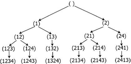
References An Heuristic Approach to Solving the one-to-one Pickup and Delivery Problem with Three-dimensional Loading Constraints
- B. Golden, S. Raghavan, and E. Wasil, The vehicle routing problem: latest advances and new challenges. Springer Science & Business Media, 2008.
- V. Pillac, M. Gendreau, C. Guéret, and A. L. Medaglia, “A review of dynamic vehicle routing problems,” European Journal of Operational Research, vol. 225, no. 1, pp. 1–11, Feb. 2013.
- S. Kumar and R. Panneerselvam, “A survey on the vehicle routing problem and its variants,” Intelligent Information Management, vol. 4, no. 3, p. 66, 2012.
- M. Gendreau, M. Iori, G. Laporte, and S. Martello, “A Tabu Search Algorithm for a Routing and Container Loading Problem,” Transportation Science, vol. 40, no. 3, pp. 342–350, Aug. 2006.
- M. Iori and S. Martello, “Routing problems with loading constraints,” TOP, vol. 18, no. 1, pp. 4–27, Jul. 2010.
- H. Pollaris, K. Braekers, A. Caris, G. K. Janssens, and S. Limbourg, “Vehicle routing problems with loading constraints: state-of-the-art and future directions,” OR Spectrum, vol. 37, no. 2, pp. 297–330, Mar. 2015.
- S. N. Parragh, K. F. Doerner, and R. F. Hartl, “A survey on pickup and delivery problems,” Journal für Betriebswirtschaft, vol. 58, no. 1, pp. 21–51, Apr. 2008.
- G. Berbeglia, J.-F. Cordeau, I. Gribkovskaia, and G. Laporte, “Static pickup and delivery problems: a classification scheme and survey,” TOP, vol. 15, no. 1, pp. 1–31, May 2007.
- J. Cordeau, G. Laporte, and S. Ropke, “Recent models and algorithms for one-to-one pickup and delivery problems,” in The vehicle routing problem: latest advances and new challenges, vol. 43, 2008, pp. 327–357.
- M. W. P. Savelsbergh and M. Sol, “The General Pickup and Delivery Problem,” Transportation Science, vol. 29, no. 1, pp. 17–29, Feb. 1995.
- S. Ropke, J.-F. Cordeau, and G. Laporte, “Models and branch-and-cut algorithms for pickup and delivery problems with time windows,” Networks, vol. 49, no. 4, pp. 258–272, 2007.
- P. Toth and D. Vigo, Vehicle routing: problems, methods, and applications. Society for Industrial and Applied Mathematics, 2014.
- W. P. Nanry and J. Wesley Barnes, “Solving the pickup and delivery problem with time windows using reactive tabu search,” Transportation Research Part B: Methodological, vol. 34, no. 2, pp. 107–121, Feb. 2000.
- H. Li and A. Lim, “A Metaheuristic for the Pickup and Delivery Problem with Time Windows,” International Journal on Artificial Intelligence Tools, vol. 12, no. 2, pp. 173–186, Jun. 2003.
- H. Lim, A. Lim, and B. Rodrigues, “Solving the pickup and delivery problem with time windows using issqueaky wheelli optimization with local search,” AMCIS 2002 Proceedings, p. 317, 2002.
- G. Pankratz, “A Grouping Genetic Algorithm for the Pickup and Delivery Problem with Time Windows,” OR Spectrum, vol. 27, no. 1, pp. 21–41, Jan. 2005.
- Q. Lu and M. M. Dessouky, “A new insertion-based construction heuristic for solving the pickup and delivery problem with time windows,” European Journal of Operational Research, vol. 175, no. 2, pp. 672–687, Dec. 2006.
- R. Bent and P. Van Hentenryck, “A two-stage hybrid algorithm for pickup and delivery vehicle routing problems with time windows,” Computers & Operations Research, vol. 33, no. 4, pp. 875–893, Apr. 2006.
- S. Ropke and D. Pisinger, “An Adaptive Large Neighborhood Search Heuristic for the Pickup and Delivery Problem with Time Windows,” Transportation Science, vol. 40, no. 4, pp. 455–472, Nov. 2006.
- Y. Nagata and S. Kobayashi, “A Memetic Algorithm for the Pickup and Delivery Problem with Time Windows Using Selective Route Exchange Crossover,” in Parallel Problem Solving from Nature, PPSN XI, Berlin, Heidelberg: Springer Berlin Heidelberg, 2010, pp. 536–545.
- J.-F. Côté, M. Gendreau, and J.-Y. Potvin, “Large neighborhood search for the pickup and delivery traveling salesman problem with multiple stacks,” Networks, vol. 60, no. 1, pp. 19–30, Aug. 2012.
- G. Erdoğan, J.-F. Cordeau, and G. Laporte, “The pickup and delivery traveling salesman problem with first-in-first-out loading,” Computers & Operations Research, vol. 36, no. 6, pp. 1800–1808, Jun. 2009.
- A. Malapert, C. Guéret, and N. Jussien, “Two-dimensional pickup and delivery routing problem with loading constraints,” in First CPAIOR Workshop on Bin Packing and Placement Constraints (BPPC’08), 2008.
- E. E. Zachariadis, C. D. Tarantilis, and C. T. Kiranoudis, “The Pallet-Packing Vehicle Routing Problem,” Transportation Science, vol. 46, no. 3, pp. 341–358, Aug. 2012.
- D. Männel and A. Bortfeldt, “A hybrid algorithm for the vehicle routing problem with pickup and delivery and three-dimensional loading constraints,” European Journal of Operational Research, vol. 254, no. 3, pp. 840–858, Nov. 2016.
- T. Bartók and C. Imreh, “Pickup and Delivery Vehicle Routing with Multidimensional Loading Constraints,” Acta Cybernetica, vol. 20, no. 1, pp. 17–33, 2011.
- D. Pisinger and S. Ropke, “A general heuristic for vehicle routing problems,” Computers & Operations Research, vol. 34, no. 8, pp. 2403–2435, Aug. 2007.
- G. Scheithauer, Y. G. Stoyan, and T. Y. Romanova, “Mathematical Modeling of Interactions of Primary Geometric 3D Objects,” Cybernetics and Systems Analysis, vol. 41, no. 3, pp. 332–342, May 2005.
- I. V. Grebennik, A. V. Pankratov, A. M. Chugay, and A. V. Baranov, “Packing n-dimensional parallelepipeds with the feasibility of changing their orthogonal orientation in an n-dimensional parallelepiped,” Cybernetics and Systems Analysis, vol. 46, no. 5, pp. 793–802, Sep. 2010.
- S. K. Ali, Z. Naser Azeez, and A. Abdul-Hussein Ouda, “A New Clustering Algorithm for Face Classification,” International Journal of Information Technology and Computer Science (IJITCS), vol. 8, no. 6, pp. 1–8, 2016.
- J. A. Hartigan and M. A. Wong, “Algorithm AS 136: A K-Means Clustering Algorithm,” Applied Statistics, vol. 28, no. 1, p. 100, 1979.
- A. C. Fabregas, B. D. Gerardo, and B. T. Tanguilig III, “Enhanced Initial Centroids for K-means Algorithm,” International Journal of Information Technology and Computer Science (IJITCS), vol. 9, no. 1, pp. 26–33, 2017.
- A. Chadha and S. Kumar, “Extension of K-Modes Algorithm for Generating Clusters Automatically,” International Journal of Information Technology and Computer Science (IJITCS), vol. 8, no. 3, pp. 51–57, 2016.
- Y. Stoyan and I. Grebennik, “Description and Generation of Combinatorial Sets Having Special Characteristics(Bilevel Programming, Optimization Methods, and Applications to Economics),” Biomedical fuzzy and human sciences : the official journal of the Biomedical Fuzzy Systems Association, vol. 18, no. 1, pp. 83–88, 2013.
- I. V. Grebennik and O. S. Lytvynenko, “Generating combinatorial sets with given properties,” Cybernetics and Systems Analysis, vol. 48, no. 6, 2012.
- B. T. Lowerre, “The HARPY Speech Recognition System.” Carnegie Mellon University, 1976.
- I. Sabuncuoglu and M. Bayiz, “Job shop scheduling with beam search,” European Journal of Operational Research, vol. 118, no. 2, pp. 390–412, Oct. 1999.
- J. Renaud, F. F. Boctor, and J. Ouenniche, “A heuristic for the pickup and delivery traveling salesman problem,” Computers & Operations Research, vol. 27, no. 9, pp. 905–916, Aug. 2000.
- S. Ropke and J.-F. Cordeau, “Branch and Cut and Price for the Pickup and Delivery Problem with Time Windows,” Transportation Science, vol. 43, no. 3, pp. 267–286, Aug. 2009.
- I. Grebennik, O. Lytvynenko, and O. Titova, “Optimization of linear function on a set of cyclic permutations,” Bionics of intellect, vol. 2, no. 67, 2012.
